Solve the system of equations through the matrix online. inverse matrix

Matrix method SLAE solutions are applied to the solution of systems of equations in which the number of equations corresponds to the number of unknowns. The method is best used for solving low-order systems. The matrix method for solving systems of linear equations is based on the application of the properties of matrix multiplication.

This way, in other words inverse matrix method, is called so, since the solution is reduced to the usual matrix equation, for the solution of which you need to find the inverse matrix.

Matrix solution method A SLAE with determinant greater than or less than zero is as follows:

Suppose there is an SLE (system of linear equations) with n unknowns (over an arbitrary field):

Hence, it is easy to translate it into matrix form:

AX = B, where A- the main matrix of the system, B and X- columns of free members and solutions of the system, respectively:

We multiply this matrix equation on the left by A −1- matrix inverse to matrix A: A −1 (AX) = A −1 B.

Because A −1 A = E, means, X = A −1 B... The right side of the equation gives the column of solutions to the initial system. The condition for the applicability of the matrix method is the nondegeneracy of the matrix A... A necessary and sufficient condition for this is the inequality to zero of the determinant of the matrix A:

detA ≠ 0.

For homogeneous system of linear equations, i.e. if vector B = 0, the inverse rule is fulfilled: the system AX = 0 there is a nontrivial (i.e., not equal to zero) solution only when detA = 0... This connection between solutions of homogeneous and inhomogeneous systems of linear equations is called alternative to Fredholm.

Thus, the solution of the SLAE by the matrix method is performed according to the formula ... Or, the solution to the SLAE is found using inverse matrix A −1.

It is known that the square matrix A order n on the n there is an inverse A −1 only if its determinant is nonzero. Thus, the system n linear algebraic equations with n unknowns are solved by the matrix method only if the determinant of the main matrix of the system is not equal to zero.

Despite the fact that there are limitations to the possibility of using such a method and there are computational difficulties for large values of the coefficients and high-order systems, the method can be easily implemented on a computer.

An example of solving an inhomogeneous SLAE.

First, let us check whether the determinant of the coefficient matrix for the unknown SLAEs is not equal to zero.

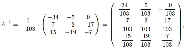
Now we find allied matrix, transpose it and substitute it into the formula for determining the inverse matrix.

Substituting the variables into the formula:

Now we find the unknowns by multiplying the inverse matrix and the column of free terms.

So, x = 2; y = 1; z = 4.

When passing from the usual form of SLAE to matrix form, be careful with the order of unknown variables in the equations of the system. for instance:

CANNOT be written as:

It is necessary, for a start, to order the unknown variables in each equation of the system and only then proceed to the matrix notation:

In addition, you need to be careful with the designation of unknown variables, instead of x 1, x 2, ..., x n there may be other letters. For example:

in matrix form, we write it like this:

It is better to use the matrix method to solve systems of linear equations in which the number of equations coincides with the number of unknown variables and the determinant of the main matrix of the system is not equal to zero. When there are more than 3 equations in the system, more computational efforts will be required to find the inverse matrix, therefore, in this case, it is advisable to use the Gaussian method for solving.

The inverse matrix method is a special case matrix equation

Solve system with matrix method

Solution: Let us write the system in matrix form and find the solution of the system by the formula (see the last formula)

We find the inverse matrix by the formula:
, where is the transposed matrix of algebraic complements of the corresponding elements of the matrix.

First, we deal with the determinant:

Here the qualifier is expanded on the first line.

Attention! If, then the inverse matrix does not exist, and it is impossible to solve the system by the matrix method. In this case, the system is solved by the method of elimination of unknowns (the Gauss method).

Now you need to calculate 9 minors and write them into the matrix of minors

Reference: It is useful to know the meaning of double subscripts in linear algebra. The first digit is the line number in which this element is located. The second digit is the number of the column in which this element is located:

That is, a double subscript indicates that the item is on the first row, third column, and, for example, the item is on row 3, column 2

In the course of the solution, it is better to describe the calculation of the minors in detail, although, with some experience, they can be accustomed to counting with errors orally.

The order of calculating the minors is not at all important, here I calculated them from left to right line by line. It was possible to calculate the minors by columns (this is even more convenient).

In this way:

- the matrix of the minors of the corresponding elements of the matrix.

- matrix of algebraic complements.

- transposed matrix of algebraic complements.

I repeat, the steps we performed were analyzed in detail in the lesson. How do I find the inverse of a matrix?

Now we write the inverse of the matrix:

In no case do we introduce into the matrix, this will seriously complicate further calculations... The division would have to be performed if all the numbers in the matrix were divisible by 60 without a remainder. But in this case, it is very necessary to introduce a minus into the matrix; on the contrary, it will simplify further calculations.

It remains to carry out matrix multiplication. You can learn how to multiply matrices in the lesson Matrix operations... By the way, exactly the same example is analyzed there.

Note that division by 60 is done in the last place.
Sometimes it may not be completely divided, i.e. "bad" fractions may result. What to do in such cases, I already told when we analyzed Cramer's rule.

Answer:

Example 12

Solve the system using the inverse matrix.

This is an example for an independent solution (a sample of finishing and the answer at the end of the lesson).

The most universal way to solve the system is method of elimination of unknowns (Gauss method)... It is not so easy to explain the algorithm easily, but I tried !.

Wish you success!

Answers:

Example 3:

Example 6:

Example 8: , ... You can view or download a sample solution for this example (link below).

Examples 10, 12:

We continue to consider systems of linear equations. This lesson is the third on the topic. If you have a vague idea of what a system of linear equations is in general, you feel like a teapot, then I recommend starting from the basics on the page Further it is useful to study the lesson.

Gauss's method is easy! Why? The famous German mathematician Johann Karl Friedrich Gauss during his lifetime was recognized as the greatest mathematician of all time, a genius and even the nickname "king of mathematics". And everything ingenious, as you know, is simple! By the way, not only fuckers, but also geniuses get paid for money - Gauss's portrait was on the 10 Deutschmark banknote (before the introduction of the euro), and Gauss still smiles mysteriously at the Germans from ordinary postage stamps.

The Gauss method is simple in that the knowledge of a 5-grade student is ENOUGH to master it. You must be able to add and multiply! It is no coincidence that teachers often consider the method of successive elimination of unknowns at school math electives. Paradoxically, the Gauss method is the most difficult for students. No wonder - the whole point is in the methodology, and I will try to tell you about the algorithm of the method in an accessible form.

First, let's systematize the knowledge about systems of linear equations a little. A system of linear equations can:

1) Have a unique solution.
2) Have infinitely many solutions.
3) Have no solutions (be inconsistent).

Gaussian method is the most powerful and versatile tool for finding a solution any systems of linear equations. As we remember Cramer's rule and matrix method unsuitable in cases where the system has infinitely many solutions or is incompatible. And the method of successive elimination of unknowns anyway will lead us to the answer! In this lesson, we will again consider the Gauss method for case No. 1 (the only solution to the system), an article is reserved for the situation of points No. 2-3. Note that the algorithm of the method itself works the same in all three cases.

Let's go back to the simplest system from the lesson How to solve a system of linear equations?
and solve it by the Gauss method.

At the first stage, you need to write extended system matrix:
... On what principle the coefficients are written, I think everyone can see. The vertical bar inside the matrix does not carry any mathematical meaning - it is just an underline for ease of design.

Reference: I recommend to rememberterms linear algebra.System Matrix Is a matrix composed only of the coefficients with unknowns, in this example the matrix of the system: . Extended system matrix - this is the same matrix of the system plus a column of free members, in this case: ... Any of the matrices can be called simply a matrix for brevity.

After the expanded matrix system is recorded, it is necessary to perform some actions with it, which are also called elementary transformations.

There are the following elementary transformations:

1) Strings matrices can be rearranged places. For example, in the matrix under consideration, you can painlessly rearrange the first and second rows:

2) If the matrix contains (or appears) proportional (as a special case - the same) rows, then it follows delete from the matrix all these rows except one. Consider, for example, the matrix ... In this matrix, the last three rows are proportional, so it is enough to leave only one of them: .

3) If a zero row appeared in the matrix during the transformations, then it also follows delete... I will not draw, of course, the zero line is the line in which only zeros.

4) The row of the matrix can be multiply (divide) by any number, nonzero... Consider, for example, a matrix. Here it is advisable to divide the first line by –3, and multiply the second line by 2: ... This action is very useful as it simplifies further matrix transformations.

5) This transformation is the most difficult, but in fact, there is nothing complicated either. To a row of a matrix, you can add another string multiplied by a number nonzero. Consider our matrix from a practical example:. First, I'll describe the conversion in great detail. Multiply the first line by –2: , and to the second line add the first line multiplied by –2:. Now the first line can be split "back" by –2:. As you can see, the line that ADD LEE – has not changed. Is always changes the line TO WHICH THE INCREASE UT.

In practice, of course, they do not describe in such detail, but write shorter:

Once again: to the second line added the first line multiplied by –2... The string is usually multiplied orally or on a draft, while the mental course of the calculations is something like this:

"Rewriting the matrix and rewriting the first line:"

“First column first. At the bottom, I need to get zero. Therefore, I multiply the unit at the top by –2:, and add the first to the second line: 2 + (–2) = 0. I write the result into the second line: »

“Now for the second column. Above –1 multiplied by –2:. I add the first to the second line: 1 + 2 = 3. I write the result into the second line: "

“And the third column. Above –5 multiplied by –2:. I add the first to the second line: –7 + 10 = 3. I write the result into the second line: »

Please, carefully comprehend this example and understand the sequential algorithm of calculations, if you understand this, then the Gauss method is practically "in your pocket". But, of course, we will work on this transformation.

Elementary transformations do not change the solution of the system of equations

! ATTENTION: considered manipulations can not use, if you are offered a task where the matrices are given "by themselves". For example, with "classic" actions with matrices In no case should you rearrange something inside the matrices!

Let's go back to our system. It has almost been solved.

We write down the extended matrix of the system and, using elementary transformations, reduce it to stepped view:

(1) The first line multiplied by –2 was added to the second line. By the way, why do we multiply the first line by –2? In order to get zero at the bottom, which means get rid of one variable in the second line.

(2) Divide the second row by 3.

The goal of elementary transformations– bring the matrix to a stepped form: ... In the design of the assignment, the "ladder" is marked out with a simple pencil, and the numbers that are located on the "steps" are circled. The term "step type" itself is not entirely theoretical; in scientific and educational literature it is often called trapezoidal view or triangular view.

As a result of elementary transformations, we obtained equivalent original system of equations:

Now the system needs to be "unrolled" in the opposite direction - from bottom to top, this process is called backward Gaussian method.

In the lower equation, we already have a ready-made result:.

Let us consider the first equation of the system and substitute the already known value of "game" into it:

Let us consider the most common situation when the Gauss method requires solving a system of three linear equations with three unknowns.

Example 1

Solve the system of equations by the Gauss method:

Let's write down the extended matrix of the system:

Now I will immediately draw the result that we will come to in the course of the solution:

And again, our goal is to bring the matrix to a stepped form using elementary transformations. Where to start the action?

First, we look at the top-left number:

It should almost always be here unit... Generally speaking, –1 will be fine (and sometimes other numbers), but somehow it so traditionally happened that the unit is usually placed there. How to organize a unit? We look at the first column - we have a ready-made unit! First transformation: swap the first and third lines:

Now the first line will remain unchanged until the end of the solution.... Now fine.

The unit in the upper left is organized. Now you need to get zeros in these places:

We get the zeros just with the help of the "difficult" transformation. First, we deal with the second line (2, –1, 3, 13). What should be done to get zero in the first position? Need to to the second line add the first line multiplied by –2... Mentally or on a draft, multiply the first line by –2: (–2, –4, 2, –18). And we consistently carry out (again mentally or on a draft) addition, to the second line we add the first line, already multiplied by –2:

We write the result to the second line:

We deal with the third line in the same way (3, 2, –5, –1). To get zero in the first position, you need to the third line add the first line multiplied by –3... Mentally or on a draft, multiply the first line by –3: (–3, –6, 3, –27). AND to the third line add the first line multiplied by –3:

We write the result in the third line:

In practice, these actions are usually performed orally and recorded in one step:

You don't need to count everything at once and at the same time... The order of calculations and "writing" the results consistent and usually like this: first we rewrite the first line, and we puff ourselves on the sly - SEQUENTIAL and CAREFULLY:

And I have already examined the mental course of the calculations themselves above.

In this example, this is easy to do, the second line is divided by –5 (since all numbers are divisible by 5 without remainder). At the same time, we divide the third line by –2, because the smaller the numbers, the easier the solution:

At the final stage of elementary transformations, you need to get another zero here:

For this to the third line add the second line multiplied by –2:

Try to parse this action yourself - mentally multiply the second line by –2 and add.

The last performed action is the hairstyle of the result, divide the third line by 3.

As a result of elementary transformations, an equivalent initial system of linear equations was obtained:

Cool.

The reverse of the Gaussian method now comes into play. The equations "unwind" from bottom to top.

In the third equation, we already have a ready-made result:

We look at the second equation:. The meaning of "z" is already known, thus:

And finally, the first equation:. "Y" and "z" are known, the matter is small:

Answer:

As has already been noted many times, for any system of equations it is possible and necessary to check the solution found, fortunately, it is easy and fast.

Example 2

This is a do-it-yourself sample, a finishing sample, and the answer at the end of the tutorial.

It should be noted that your decision course may not coincide with my course of decision, and this is a feature of the Gauss method... But the answers must be the same!

Example 3

Solve a system of linear equations by the Gaussian method

Let us write down the extended matrix of the system and, using elementary transformations, bring it to a stepwise form:

We look at the upper left "step". We should have a unit there. The problem is that there are no ones in the first column at all, so rearranging the rows will not solve anything. In such cases, the unit needs to be organized using an elementary transformation. This can usually be done in several ways. I did this: (1) To the first line add the second line multiplied by -1... That is, we mentally multiplied the second line by –1 and added the first and second lines, while the second line did not change.

Now the top left is -1, which is fine for us. Anyone who wants to get +1 can perform an additional body movement: multiply the first line by –1 (change its sign).

(2) The first line multiplied by 5 was added to the second line. The first line multiplied by 3 was added to the third line.

(3) The first line was multiplied by -1, in principle, this is for beauty. We also changed the sign of the third line and moved it to the second place, thus, on the second “step, we have the required unit.

(4) The second row, multiplied by 2, was added to the third row.

(5) The third line was divided by 3.

A bad sign that indicates an error in calculations (less often - a typo) is the "bad" bottom line. That is, if at the bottom we got something like, and, accordingly, , then with a high degree of probability it can be argued that a mistake was made in the course of elementary transformations.

We charge the reverse stroke, in the design of examples, the system itself is often not rewritten, and the equations "are taken directly from the given matrix." The reverse move, I remind you, works, from the bottom up:
Yes, here the gift turned out:

Answer: .

Example 4

Solve a system of linear equations by the Gaussian method

This is an example for an independent solution, it is somewhat more complicated. It's okay if anyone gets confused. Complete solution and sample design at the end of the tutorial. Your solution may differ from mine.

In the last part, we will consider some of the features of the Gauss algorithm.
The first feature is that sometimes some variables are missing in the equations of the system, for example:

How to write the extended system matrix correctly? I already talked about this moment in the lesson. Cramer's rule. Matrix method... In the extended matrix of the system, we put zeros in place of the missing variables:

By the way, this is a fairly easy example, since there is already one zero in the first column, and there are fewer elementary transformations to be performed.

The second feature is as follows. In all the considered examples, we placed either –1 or +1 on the “steps”. Could other numbers be there? In some cases, they can. Consider the system: .

Here, on the upper left "step" we have a two. But we notice the fact that all the numbers in the first column are divisible by 2 without a remainder - and the other two and six. And the deuce at the top left will suit us! At the first step, you need to perform the following transformations: add the first line multiplied by –1 to the second line; to the third line add the first line multiplied by –3. This will give us the desired zeros in the first column.

Or another conditional example: ... Here the three on the second "step" also suits us, since 12 (the place where we need to get zero) is divisible by 3 without a remainder. It is necessary to carry out the following transformation: to the third line add the second line multiplied by –4, as a result of which the zero we need will be obtained.

Gauss's method is universal, but there is one peculiarity. You can confidently learn how to solve systems by other methods (Cramer's method, matrix method) literally the first time - there is a very rigid algorithm. But in order to feel confident in the Gauss method, you should "fill your hand" and solve at least 5-10 ten systems. Therefore, at first, confusion, errors in calculations are possible, and there is nothing unusual or tragic in this.

Rainy autumn weather outside the window ... Therefore, for everyone, a more complex example for an independent solution:

Example 5

Solve the system of 4 linear equations with four unknowns by the Gauss method.

Such a task in practice is not so rare. I think that even a teapot who has thoroughly studied this page, the algorithm for solving such a system is intuitively clear. Basically, everything is the same - there are just more actions.

Cases when the system has no solutions (inconsistent) or has infinitely many solutions are considered in the lesson Incompatible systems and systems with a common solution... The considered algorithm of the Gauss method can also be fixed there.

Wish you success!

Solutions and Answers:

Example 2: Let us write down the extended matrix of the system and, using elementary transformations, bring it to a stepwise form.

Elementary transformations performed:
(1) The first line multiplied by –2 was added to the second line. The first line multiplied by -1 was added to the third line.Attention! Here it may be tempting to subtract the first from the third line, I highly discourage subtracting - the risk of an error is greatly increased. Just add up!
(2) The sign of the second line was changed (multiplied by –1). The second and third lines were swapped.note that on the "steps" we are satisfied with not only one, but also –1, which is even more convenient.
(3) The second row was added to the third row, multiplied by 5.
(4) The sign of the second line was changed (multiplied by –1). The third line was split by 14.

Reverse:

Answer: .

Example 4: We write down the extended matrix of the system and, using elementary transformations, bring it to a stepwise form:

Conversions performed:
(1) The second was added to the first line. Thus, the desired unit is organized on the upper left "rung".
(2) The first line multiplied by 7 was added to the second line. The first line multiplied by 6 was added to the third line.

The second step is getting worse , "Candidates" for it are the numbers 17 and 23, and we need either one or -1. Transformations (3) and (4) will be aimed at obtaining the desired unit

(3) The second line was added to the third line, multiplied by –1.
(4) The third line was added to the second line, multiplied by –3.
The necessary thing on the second step is received .
(5) The second line was added to the third line, multiplied by 6.
(6) The second line was multiplied by -1, the third line was divided by -83. It is obvious that the plane is uniquely determined by three different points that do not lie on one straight line. Therefore, three-letter designations of planes are quite popular - by points belonging to them, for example,; .If free members

In the first part, we considered a little theoretical material, the substitution method, and also the method of term-by-term addition of the equations of the system. I recommend to everyone who came to the site through this page to read the first part. Perhaps some visitors will find the material too simple, but in the course of solving systems of linear equations, I made a number of very important remarks and conclusions concerning the solution of mathematical problems in general.

And now we will analyze Cramer's rule, as well as solving a system of linear equations using an inverse matrix (matrix method). All materials are presented in a simple, detailed and understandable way, almost all readers will be able to learn how to solve systems in the above ways.

First, we consider in detail Cramer's rule for a system of two linear equations in two unknowns. What for? - After all, the simplest system can be solved by the school method, the method of term-by-term addition!

The fact is that, even if sometimes, such a task is encountered - to solve a system of two linear equations with two unknowns according to Cramer's formulas. Second, a simpler example will help you understand how to use Cramer's rule for a more complex case - a system of three equations with three unknowns.

In addition, there are systems of linear equations with two variables, which it is advisable to solve exactly according to Cramer's rule!

Consider the system of equations

At the first step, we calculate the determinant, it is called main determinant of the system.

Gauss method.

If, then the system has a unique solution, and to find the roots, we must calculate two more determinants:
and

In practice, the above qualifiers can also be denoted by a Latin letter.

We find the roots of the equation by the formulas:
,

Example 7

Solve a system of linear equations

Solution: We see that the coefficients of the equation are large enough, on the right side there are decimal fractions with a comma. The comma is a rather rare guest in practical exercises in mathematics; I took this system from an econometric problem.

How to solve such a system? You can try to express one variable in terms of another, but in this case you will surely get terrible fancy fractions, which are extremely inconvenient to work with, and the design of the solution will look just awful. You can multiply the second equation by 6 and perform term-by-term subtraction, but the same fractions will appear here.

What to do? In such cases, Cramer's formulas come to the rescue.

;

Answer: ,

Both roots have infinite tails, and are found approximately, which is quite acceptable (and even common) for econometric problems.

Comments are not needed here, since the task is solved according to ready-made formulas, however, there is one caveat. When using this method, compulsory a fragment of the assignment is the following fragment: "Which means that the system has the only solution"... Otherwise, the reviewer may punish you for disrespecting Cramer's theorem.

It will not be superfluous to check, which is convenient to carry out on a calculator: we substitute approximate values into the left side of each equation in the system. As a result, with a small error, you should get numbers that are in the right parts.

Example 8

The answer is presented in ordinary irregular fractions. Make a check.

This is an example for an independent solution (example of finishing and the answer at the end of the lesson).

We now turn to the consideration of Cramer's rule for a system of three equations with three unknowns:

Find the main determinant of the system:

If, then the system has infinitely many solutions or is inconsistent (has no solutions). In this case, Cramer's rule will not help; you need to use the Gaussian method.

If, then the system has a unique solution, and to find the roots, we must calculate three more determinants:
, ,

And finally, the answer is calculated using the formulas:

As you can see, the case "three by three" is fundamentally no different from the case "two by two", the column of free members sequentially "walks" from left to right along the columns of the main determinant.

Example 9

Solve the system using Cramer's formulas.

Solution: Let's solve the system using Cramer's formulas.

, which means that the system has a unique solution.

Answer: .

Actually, there is nothing special to comment on here again, in view of the fact that the decision is made according to ready-made formulas. But there are a couple of things to note.

It so happens that as a result of calculations "bad" irreducible fractions are obtained, for example:.
I recommend the following "cure" algorithm. If you don't have a computer at hand, we do this:

1) There may be a calculation error. As soon as you are faced with a "bad" fraction, you should immediately check is the condition rewritten correctly... If the condition is rewritten without errors, then it is necessary to recalculate the determinants using the expansion by another row (column).

2) If no errors were found as a result of checking, then most likely there was a typo in the task condition. In this case, calmly and CAREFULLY we solve the task to the end, and then be sure to check and make it out on a clean copy after the decision. Of course, checking a fractional answer is an unpleasant lesson, but it will be a disarming argument for a teacher who, well, very much loves to put a minus for any byaka like. How to handle fractions is detailed in the answer for Example 8.

If you have a computer at hand, then use an automated program to check it, which can be downloaded for free at the very beginning of the lesson. By the way, it is most profitable to use the program right away (even before starting the solution), you will immediately see the intermediate step at which you made a mistake! The same calculator automatically calculates the solution of the system by the matrix method.

Second remark. From time to time, there are systems in the equations of which some variables are missing, for example:

Here, the first equation is missing a variable, the second is missing a variable. In such cases, it is very important to correctly and CAREFULLY write down the main determinant:
- zeros are put in place of missing variables.
By the way, it is rational to open determinants with zeros according to the row (column) in which there is zero, since the calculations are much less.

Example 10

Solve the system using Cramer's formulas.

This is an example for an independent solution (a sample of finishing and the answer at the end of the lesson).

For the case of a system of 4 equations with 4 unknowns, Cramer's formulas are written according to similar principles. A live example can be found in the Determinant Properties lesson. Lowering the order of the determinant - five determinants of the 4th order are quite solvable. Although the task is already quite reminiscent of the professor's boot on the chest of a lucky student.

Solving the system using the inverse matrix

The inverse matrix method is essentially a special case matrix equation(see Example # 3 of the specified lesson).

To study this section, you must be able to expand determinants, find the inverse matrix, and perform matrix multiplication. Relevant links will be provided along the way.

Example 11

Solve system with matrix method

Solution: Let's write the system in matrix form:
, where

Please take a look at the system of equations and the matrices. By what principle we write elements into matrices, I think everyone understands. The only comment: if some variables were missing in the equations, then zeros would have to be put in the corresponding places in the matrix.

We find the inverse matrix by the formula:
, where is the transposed matrix of algebraic complements of the corresponding elements of the matrix.

First, we deal with the determinant:

Here the qualifier is expanded on the first line.

Now you need to calculate 9 minors and write them into the matrix of minors

This online calculator solves a system of linear equations by the matrix method. A very detailed solution is given. Select the number of variables to solve a system of linear equations. Choose a method for calculating the inverse matrix. Then enter the data in the cells and click on the "Calculate" button.

Warning

Clear all cells?

Close Clear

Data entry instructions. Numbers are entered as whole numbers (examples: 487, 5, -7623, etc.), decimal numbers (eg 67., 102.54, etc.) or fractions. The fraction must be typed in the form a / b, where a and b are integers or decimal numbers. Examples 45/5, 6.6 / 76.4, -7 / 6.7, etc.

Matrix method for solving systems of linear equations

Consider the following system of linear equations:

Taking into account the definition of the inverse matrix, we have A −1 A=E, where E is the identity matrix. Therefore (4) can be written as follows:

Thus, to solve the system of linear equations (1) (or (2)), it is sufficient to multiply the inverse to A matrix by vector of constraints b.

Examples of solving a system of linear equations by the matrix method

Example 1. Solve the following system of linear equations by the matrix method:

Let us find the inverse of the matrix A by the Jordan-Gauss method. On the right side of the matrix A we write the identity matrix:

Eliminate the elements of the 1st column of the matrix below the main diagonal. To do this, add rows 2,3 with row 1 multiplied by -1 / 3, -1 / 3, respectively:

Eliminate the elements of the 2nd column of the matrix below the main diagonal. To do this, add line 3 with line 2 multiplied by -24/51:

Eliminate the elements of the 2nd column of the matrix above the main diagonal. To do this, add line 1 with line 2 multiplied by -3/17:

Separate the right side of the matrix. The resulting matrix is the inverse of the matrix to A :

Matrix form of recording a system of linear equations: Ax = b, where

We calculate all the algebraic complements of the matrix A:

The inverse matrix is calculated from the following expression.

Equations in general, linear algebraic equations and their systems, as well as methods for their solution, occupy a special place in mathematics, both theoretical and applied.

This is due to the fact that the overwhelming majority of physical, economic, technical and even pedagogical problems can be described and solved using a variety of equations and their systems. Recently, mathematical modeling has gained particular popularity among researchers, scientists and practitioners in almost all subject areas, which is explained by its obvious advantages over other known and tested methods for studying objects of various nature, in particular, so-called complex systems. There is a great variety of different definitions of the mathematical model given by scientists at different times, but in our opinion, the most successful is the following statement. A mathematical model is an idea expressed by an equation. Thus, the ability to compose and solve equations and their systems is an integral characteristic of a modern specialist.

To solve systems of linear algebraic equations, the most commonly used methods are: Cramer, Jordan-Gauss and the matrix method.

Matrix solution method - a method for solving systems of linear algebraic equations with a nonzero determinant using an inverse matrix.

If we write the coefficients for unknown values xi into the matrix A, collect the unknown quantities into a vector column X, and free terms into a vector column B, then the system of linear algebraic equations can be written in the form of the following matrix equation A X = B, which has a unique solution only when the determinant of the matrix A is not equal to zero. In this case, the solution to the system of equations can be found in the following way X = A-one · B, where A-1 is the inverse of the matrix.

The matrix solution method is as follows.

Let a system of linear equations with n unknown:

It can be rewritten in matrix form: AX = B, where A- the main matrix of the system, B and X- columns of free members and solutions of the system, respectively:

We multiply this matrix equation on the left by A-1 - matrix inverse to matrix A: A -1 (AX) = A -1 B

Because A -1 A = E, we get X= A -1 B... The right side of this equation will give the column of solutions to the original system. The condition for the applicability of this method (as well as in general for the existence of a solution to an inhomogeneous system of linear equations with the number of equations equal to the number of unknowns) is the nondegeneracy of the matrix A... A necessary and sufficient condition for this is the inequality to zero of the determinant of the matrix A: det A≠ 0.

For a homogeneous system of linear equations, that is, when the vector B = 0 , indeed the opposite is true: the system AX = 0 has a nontrivial (that is, nonzero) solution only if det A= 0. Such a connection between solutions of homogeneous and inhomogeneous systems of linear equations is called the Fredholm alternative.

Example solutions of an inhomogeneous system of linear algebraic equations.

Let us make sure that the determinant of the matrix composed of the coefficients of the unknowns of the system of linear algebraic equations is not equal to zero.

The next step is to calculate the algebraic complements for the elements of the matrix consisting of the coefficients of the unknowns. They will be needed to find the inverse matrix.