Discrete Poisson distribution. Poisson distribution
The binomial distribution law applies to cases where a sample of a fixed size was taken. The Poisson distribution applies to cases where the number of random events occurs over a certain length, area, volume or time, while the determining parameter of the distribution is the average number of events , not sample size P and probability of success R. For example, the number of nonconformities in a sample or the number of nonconformities per unit of production.
Probability distribution for number of successes X has the following form:
Or we can say that a discrete random variable X distributed according to Poisson's law if its possible values are 0.1, 2, ...t, ...p, and the probability of occurrence of such values is determined by the relation:
Where m or λ is some positive value called the Poisson distribution parameter.
Poisson's law applies to “rarely” occurring events, while the possibility of the next success (for example, a failure) persists continuously, is constant and does not depend on the number of previous successes or failures (when we are talking about processes developing over time, this is called “independence of of the past"). A classic example where Poisson's law applies is the number of telephone calls at a telephone exchange during a given time interval. Other examples might be the number of ink blots on the page of a sloppily written manuscript, or the number of specks that end up on the body of a car while painting it. The Poisson distribution law measures the number of defects, not the number of defective products.
The Poisson distribution is governed by the number of random events that occur at fixed time intervals or in a fixed region of space. For λ<1 значение P(m) монотонно убывает с ростом m то, a при λ>1 value P(m)increasing T passes through a maximum near /
A feature of the Poisson distribution is that the variance is equal to the mathematical expectation. Poisson distribution parameters
M(x) = σ 2 = λ (15)
This feature of the Poisson distribution allows us to state in practice that the experimentally obtained distribution of a random variable is subject to the Poisson distribution if the sample values of the mathematical expectation and variance are approximately equal.
The law of rare events is used in mechanical engineering for selective control of finished products, when, according to technical conditions, a certain percentage of defects (usually small) is allowed in the accepted batch of products q<<0.1.
If the probability q of event A is very small (q≤0.1), and the number of trials is large, then the probability that event A will occur m times in n trials will be equal to
where λ = M(x) = nq
To calculate the Poisson distribution, you can use the following recurrence relations
The Poisson distribution plays an important role in statistical quality assurance methods because it can be used to approximate hypergeometric and binomial distributions.
Such an approximation is acceptable when , provided that qn has a finite limit and q<0.1. Когда p →∞, A r → 0, average n r = t = const.
Using the law of rare events, you can calculate the probability that a sample of n units will contain: 0,1,2,3, etc. defective parts, i.e. given m times. You can also calculate the probability of m or more defective parts appearing in such a sample. This probability, based on the rule of adding probabilities, will be equal to:
Example 1. The batch contains defective parts, the proportion of which is 0.1. 10 parts are taken sequentially and examined, after which they are returned to the batch, i.e. the tests are independent. What is the probability that when checking 10 parts, one will be defective?
Solution From the problem conditions q=0.1; n=10; m=1.Obviously, p=1-q=0.9.
The result obtained can also be applied to the case when 10 parts are removed in a row without returning them back to the batch. With a large enough batch, for example, 1000 pieces, the probability of extracting parts will change negligibly. Therefore, under such conditions, the removal of a defective part can be considered as an event that does not depend on the results of previous tests.
Example 2. The batch contains 1% defective parts. What is the probability that, when taking a sample of 50 units of product from a batch, it will contain 0, 1, 2, 3, 4 defective parts?
Solution. Here q=0.01, nq=50*0.01=0.5
Thus, to effectively use the Poisson distribution as an approximation of the binomial, it is necessary that the probability of success R was significantly less q. a n r = t was of the order of one (or several units).
Thus, in statistical quality assurance methods
hypergeometric law applicable for samples of any size P and any level of non-conformity q ,
binomial law and Poisson's law are its special cases, respectively, provided that n/N<0,1 и
The most common case of various types of probability distributions is the binomial distribution. Let us use its versatility to determine the most common particular types of distributions encountered in practice.
Binomial distribution
Let there be some event A. The probability of occurrence of event A is equal to p, the probability of non-occurrence of event A is 1 p, sometimes it is designated as q. Let n number of tests, m frequency of occurrence of event A in these n tests.
It is known that the total probability of all possible combinations of outcomes is equal to one, that is:
1 = p n + n · p n 1 (1 p) + C n n 2 · p n 2 (1 p) 2 + + C n m · p m· (1 p) n m+ + (1 p) n .
|
p n probability that in nn once; n · p n 1 (1 p) probability that in nn 1) once and will not happen 1 time; C n n 2 · p n 2 (1 p) 2 probability that in n tests, event A will occur ( n 2) times and will not happen 2 times; P m = C n m · p m· (1 p) n m probability that in n tests, event A will occur m will never happen ( n m) once; (1 p) n probability that in n in trials, event A will not occur even once; number of combinations of n By m . |
Expected value M binomial distribution is equal to:
M = n · p ,
Where n number of tests, p probability of occurrence of event A.
Standard deviation σ :
σ = sqrt( n · p· (1 p)) .
Example 1. Calculate the probability that an event that has a probability p= 0.5, in n= 10 trials will happen m= 1 time. We have: C 10 1 = 10, and further: P 1 = 10 0.5 1 (1 0.5) 10 1 = 10 0.5 10 = 0.0098. As we can see, the probability of this event occurring is quite low. This is explained, firstly, by the fact that it is absolutely not clear whether the event will happen or not, since the probability is 0.5 and the chances here are “50 to 50”; and secondly, it is required to calculate that the event will occur exactly once (no more and no less) out of ten.
Example 2. Calculate the probability that an event that has a probability p= 0.5, in n= 10 trials will happen m= 2 times. We have: C 10 2 = 45, and further: P 2 = 45 0.5 2 (1 0.5) 10 2 = 45 0.5 10 = 0.044. The likelihood of this event occurring has increased!
Example 3. Let's increase the likelihood of the event itself occurring. Let's make it more likely. Calculate the probability that an event that has a probability p= 0.8, in n= 10 trials will happen m= 1 time. We have: C 10 1 = 10, and further: P 1 = 10 0.8 1 (1 0.8) 10 1 = 10 0.8 1 0.2 9 = 0.000004. The probability has become less than in the first example! The answer, at first glance, seems strange, but since the event has a fairly high probability, it is unlikely to happen only once. It is more likely that it will happen more than once. Indeed, counting P 0 , P 1 , P 2 , P 3, , P 10 (probability that an event in n= 10 trials will happen 0, 1, 2, 3, , 10 times), we will see:
C 10 0 = 1
,
C 10 1 = 10
,
C 10 2 = 45
,
C 10 3 = 120
,
C 10 4 = 210
,
C 10 5 = 252
,
C 10 6 = 210
,
C 10 7 = 120
,
C 10 8 = 45
,
C 10 9 = 10
,
C 10 10 = 1
;
P 0 = 1 0.8 0 (1 0.8) 10 0 = 1 1 0.2 10 = 0.0000;
P 1 = 10 0.8 1 (1 0.8) 10 1 = 10 0.8 1 0.2 9 = 0.0000;
P 2 = 45 0.8 2 (1 0.8) 10 2 = 45 0.8 2 0.2 8 = 0.0000;
P 3 = 120 0.8 3 (1 0.8) 10 3 = 120 0.8 3 0.2 7 = 0.0008;
P 4 = 210 0.8 4 (1 0.8) 10 4 = 210 0.8 4 0.2 6 = 0.0055;
P 5 = 252 0.8 5 (1 0.8) 10 5 = 252 0.8 5 0.2 5 = 0.0264;
P 6 = 210 0.8 6 (1 0.8) 10 6 = 210 0.8 6 0.2 4 = 0.0881;
P 7 = 120 0.8 7 (1 0.8) 10 7 = 120 0.8 7 0.2 3 = 0.2013;
P 8 = 45 0.8 8 (1 0.8) 10 8 = 45 0.8 8 0.2 2 = 0.3020(highest probability!);
P 9 = 10 0.8 9 (1 0.8) 10 9 = 10 0.8 9 0.2 1 = 0.2684;
P 10 = 1 0.8 10 (1 0.8) 10 10 = 1 0.8 10 0.2 0 = 0.1074
Of course P 0 + P 1 + P 2 + P 3 + P 4 + P 5 + P 6 + P 7 + P 8 + P 9 + P 10 = 1 .
Normal distribution
If we depict the quantities P 0 , P 1 , P 2 , P 3, , P 10, which we calculated in example 3, on the graph, it turns out that their distribution has a form close to the normal distribution law (see Fig. 27.1) (see lecture 25. Modeling of normally distributed random variables).
probabilities for different m at p = 0.8, n = 10
The binomial law becomes normal if the probabilities of occurrence and non-occurrence of event A are approximately the same, that is, we can conditionally write: p≈ (1 p) . For example, let's take n= 10 and p= 0.5 (that is p= 1 p = 0.5 ).
We will come to such a problem meaningfully if, for example, we want to theoretically calculate how many boys and how many girls there will be out of 10 children born in a maternity hospital on the same day. More precisely, we will count not boys and girls, but the probability that only boys will be born, that 1 boy and 9 girls will be born, that 2 boys and 8 girls will be born, and so on. Let us assume for simplicity that the probability of having a boy and a girl is the same and equal to 0.5 (but in fact, to be honest, this is not the case, see the course “Modeling Artificial Intelligence Systems”).
It is clear that the distribution will be symmetrical, since the probability of having 3 boys and 7 girls is equal to the probability of having 7 boys and 3 girls. The greatest likelihood of birth will be 5 boys and 5 girls. This probability is equal to 0.25, by the way, it is not that big in absolute value. Further, the probability that 10 or 9 boys will be born at once is much less than the probability that 5 ± 1 boy will be born out of 10 children. The binomial distribution will help us make this calculation. So.
C 10 0 = 1
,
C 10 1 = 10
,
C 10 2 = 45
,
C 10 3 = 120
,
C 10 4 = 210
,
C 10 5 = 252
,
C 10 6 = 210
,
C 10 7 = 120
,
C 10 8 = 45
,
C 10 9 = 10
,
C 10 10 = 1
;
P 0 = 1 0.5 0 (1 0.5) 10 0 = 1 1 0.5 10 = 0.000977;
P 1 = 10 0.5 1 (1 0.5) 10 1 = 10 0.5 10 = 0.009766;
P 2 = 45 0.5 2 (1 0.5) 10 2 = 45 0.5 10 = 0.043945;
P 3 = 120 0.5 3 (1 0.5) 10 3 = 120 0.5 10 = 0.117188;
P 4 = 210 0.5 4 (1 0.5) 10 4 = 210 0.5 10 = 0.205078;
P 5 = 252 0.5 5 (1 0.5) 10 5 = 252 0.5 10 = 0.246094;
P 6 = 210 0.5 6 (1 0.5) 10 6 = 210 0.5 10 = 0.205078;
P 7 = 120 0.5 7 (1 0.5) 10 7 = 120 0.5 10 = 0.117188;
P 8 = 45 0.5 8 (1 0.5) 10 8 = 45 0.5 10 = 0.043945;
P 9 = 10 0.5 9 (1 0.5) 10 9 = 10 0.5 10 = 0.009766;
P 10 = 1 0.5 10 (1 0.5) 10 10 = 1 0.5 10 = 0.000977
Of course P 0 + P 1 + P 2 + P 3 + P 4 + P 5 + P 6 + P 7 + P 8 + P 9 + P 10 = 1 .
Let us display the quantities on the graph P 0 , P 1 , P 2 , P 3, , P 10 (see Fig. 27.2).
p = 0.5 and n = 10, bringing it closer to the normal law
So, under the conditions m ≈ n/2 and p≈ 1 p or p≈ 0.5 instead of the binomial distribution, you can use the normal one. For large values n the graph shifts to the right and becomes more and more flat, as the mathematical expectation and variance increase with increasing n : M = n · p , D = n · p· (1 p) .
By the way, the binomial law tends to normal and with increasing n, which is quite natural, according to the central limit theorem (see lecture 34. Recording and processing statistical results).
Now consider how the binomial law changes in the case when p ≠ q, that is p> 0 . In this case, the hypothesis of normal distribution cannot be applied, and the binomial distribution becomes a Poisson distribution.
Poisson distribution
The Poisson distribution is a special case of the binomial distribution (with n>> 0 and at p>0 (rare events)).
A formula is known from mathematics that allows you to approximately calculate the value of any member of the binomial distribution:
Where a = n · p Poisson parameter (mathematical expectation), and the variance is equal to the mathematical expectation. Let us present mathematical calculations that explain this transition. Binomial distribution law
P m = C n m · p m· (1 p) n m
can be written if you put p = a/n , as
![]()
Because p is very small, then only the numbers should be taken into account m, small compared to n. Work
very close to unity. The same applies to the size
Magnitude
very close to e a. From here we get the formula:
Example. The box contains n= 100 parts, both high-quality and defective. The probability of receiving a defective product is p= 0.01 . Let's say that we take out a product, determine whether it is defective or not, and put it back. By doing this, it turned out that out of 100 products that we went through, two turned out to be defective. What is the likelihood of this?
From the binomial distribution we get:
From the Poisson distribution we get:
As you can see, the values turned out to be close, so in the case of rare events it is quite acceptable to apply Poisson’s law, especially since it requires less computational effort.
Let us show graphically the form of Poisson's law. Let's take the parameters as an example p = 0.05 , n= 10 . Then:
C 10 0 = 1
,
C 10 1 = 10
,
C 10 2 = 45
,
C 10 3 = 120
,
C 10 4 = 210
,
C 10 5 = 252
,
C 10 6 = 210
,
C 10 7 = 120
,
C 10 8 = 45
,
C 10 9 = 10
,
C 10 10 = 1
;
P 0 = 1 0.05 0 (1 0.05) 10 0 = 1 1 0.95 10 = 0.5987;
P 1 = 10 0.05 1 (1 0.05) 10 1 = 10 0.05 1 0.95 9 = 0.3151;
P 2 = 45 0.05 2 (1 0.05) 10 2 = 45 0.05 2 0.95 8 = 0.0746;
P 3 = 120 0.05 3 (1 0.05) 10 3 = 120 0.05 3 0.95 7 = 0.0105;
P 4 = 210 0.05 4 (1 0.05) 10 4 = 210 0.05 4 0.95 6 = 0.00096;
P 5 = 252 0.05 5 (1 0.05) 10 5 = 252 0.05 5 0.95 5 = 0.00006;
P 6 = 210 0.05 6 (1 0.05) 10 6 = 210 0.05 6 0.95 4 = 0.0000;
P 7 = 120 0.05 7 (1 0.05) 10 7 = 120 0.05 7 0.95 3 = 0.0000;
P 8 = 45 0.05 8 (1 0.05) 10 8 = 45 0.05 8 0.95 2 = 0.0000;
P 9 = 10 0.05 9 (1 0.05) 10 9 = 10 0.05 9 0.95 1 = 0.0000;
P 10 = 1 0.05 10 (1 0.05) 10 10 = 1 0.05 10 0.95 0 = 0.0000
Of course P 0 + P 1 + P 2 + P 3 + P 4 + P 5 + P 6 + P 7 + P 8 + P 9 + P 10 = 1 .
At n> ∞ the Poisson distribution turns into a normal law, according to the central limit theorem (see.
Let's consider the Poisson distribution, calculate its mathematical expectation, variance, and mode. Using the MS EXCEL function POISSON.DIST(), we will construct graphs of the distribution function and probability density. Let us estimate the distribution parameter, its mathematical expectation and standard deviation.
First, we give a dry formal definition of distribution, then we give examples of situations when Poisson distribution(English) Poissondistribution) is an adequate model for describing a random variable.
If random events occur in a given period of time (or in a certain volume of matter) with an average frequency λ( lambda), then the number of events x, occurred during this period of time will have Poisson distribution.
Application of the Poisson distribution
Examples when Poisson distribution is an adequate model:
- the number of calls received at the telephone exchange over a certain period of time;
- the number of particles that have undergone radioactive decay over a certain period of time;
- number of defects in a piece of fabric of a fixed length.
Poisson distribution is an adequate model if the following conditions are met:
- events occur independently of each other, i.e. the probability of a subsequent event does not depend on the previous one;
- the average event rate is constant. As a consequence, the probability of an event is proportional to the length of the observation interval;
- two events cannot happen at the same time;
- the number of events must take the value 0; 1; 2…
Note: A good clue is that the observed random variable has Poisson distribution, is the fact that it is approximately equal (see below).
Below are examples of situations where Poisson distribution can not be applied:
- the number of students who leave the university within an hour (since the average flow of students is not constant: during classes there are few students, and during the break between classes the number of students increases sharply);
- the number of earthquakes with an amplitude of 5 points per year in California (since one earthquake can cause aftershocks of similar amplitude - the events are not independent);
- the number of days that patients spend in the intensive care unit (because the number of days that patients spend in the intensive care unit is always greater than 0).
Note: Poisson distribution is an approximation of more accurate discrete distributions: and .
Note: About the relationship Poisson distribution And Binomial distribution can be read in the article. About the relationship Poisson distribution And Exponential distribution can be read in the article about.
Poisson distribution in MS EXCEL
In MS EXCEL, starting from version 2010, for Distributions Poisson there is a function POISSON.DIST(), English name - POISSON.DIST(), which allows you to calculate not only the probability that over a given period of time will happen X events (function probability density p(x), see formula above), but also (the probability that during a given period of time at least x events).
Before MS EXCEL 2010, EXCEL had the POISSON() function, which also allows you to calculate distribution function And probability density p(x). POISSON() is left in MS EXCEL 2010 for compatibility.
The example file contains graphs probability density distribution And cumulative distribution function.

Poisson distribution has a skewed shape (a long tail on the right side of the probability function), but as the parameter λ increases, it becomes more and more symmetrical.
Note: Average And dispersion(square) are equal to the parameter Poisson distribution– λ (see example sheet file Example).
Task
Typical Application Poisson distributions in quality control is a model of the number of defects that may appear in an instrument or device.
For example, with an average number of defects in a chip λ (lambda) equal to 4, the probability that a randomly selected chip will have 2 or fewer defects is: = POISSON.DIST(2,4,TRUE)=0.2381
The third parameter in the function is set = TRUE, so the function will return cumulative distribution function, that is, the probability that the number of random events will be in the range from 0 to 4 inclusive.
Calculations in this case are made according to the formula:
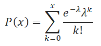
The probability that a randomly selected microcircuit will have exactly 2 defects is: = POISSON.DIST(2,4,FALSE)=0.1465
The third parameter in the function is set = FALSE, so the function will return the probability density.
The probability that a randomly selected microcircuit will have more than 2 defects is equal to: =1-POISSON.DIST(2,4,TRUE) =0.8535
Note: If x is not an integer, then when calculating the formula . Formulas =POISSON.DIST( 2 ; 4; LIE) And =POISSON.DIST( 2,9 ; 4; LIE) will return the same result.
Random number generation and λ estimation
For values of λ >15 , Poisson distribution well approximated Normal distribution with the following parameters: μ =λ , σ 2 =λ .
More details about the relationship between these distributions can be found in the article. There are also examples of approximation, and the conditions for when it is possible and with what accuracy are explained.
ADVICE: You can read about other MS EXCEL distributions in the article.
Introduction
Are random phenomena subject to any laws? Yes, but these laws differ from the physical laws we are familiar with. The values of SV cannot be predicted even under known experimental conditions; we can only indicate the probabilities that SV will take one or another value. But knowing the probability distribution of SVs, we can draw conclusions about the events in which these random variables participate. True, these conclusions will also be probabilistic in nature.
Let some SV be discrete, i.e. can only take fixed values Xi. In this case, the series of probability values P(Xi) for all (i=1…n) permissible values of this quantity is called its distribution law.
The law of distribution of SV is a relation that establishes a connection between possible values of SV and the probabilities with which these values are accepted. The distribution law fully characterizes the SV.
When constructing a mathematical model to test a statistical hypothesis, it is necessary to introduce a mathematical assumption about the law of distribution of SV (parametric way of constructing the model).
The nonparametric approach to describing the mathematical model (SV does not have a parametric distribution law) is less accurate, but has a wider scope.
Just like for the probability of a random event, for the distribution law of SV there are only two ways to find it. Either we build a diagram of a random event and find an analytical expression (formula) for calculating the probability (perhaps someone has already done or will do this for us!), or we will have to use an experiment and, based on the frequencies of observations, make some assumptions (put forward hypotheses) about the law distributions.
Of course, for each of the “classical” distributions this work has been done for a long time - widely known and very often used in applied statistics are binomial and polynomial distributions, geometric and hypergeometric, Pascal and Poisson distributions and many others.
For almost all classical distributions, special statistical tables were immediately constructed and published, refined as the accuracy of the calculations increased. Without the use of many volumes of these tables, without training in the rules for using them, the practical use of statistics has been impossible for the last two centuries.
Today the situation has changed - there is no need to store calculation data using formulas (no matter how complex the latter may be!), the time to use the distribution law for practice has been reduced to minutes, or even seconds. There are already a sufficient number of different application software packages for these purposes.
Among all probability distributions, there are those that are used especially often in practice. These distributions have been studied in detail and their properties are well known. Many of these distributions underlie entire areas of knowledge - such as queuing theory, reliability theory, quality control, game theory, etc.
Among them, one cannot help but pay attention to the works of Poisson (1781-1840), who proved a more general form of the law of large numbers than Jacob Bernoulli, and also for the first time applied the theory of probability to shooting problems. The name of Poisson is associated with one of the laws of distribution, which plays an important role in probability theory and its applications.
It is this distribution law that this course work is devoted to. We will talk directly about the law, about its mathematical characteristics, special properties, and connection with the binomial distribution. A few words will be said about practical application and several examples from practice will be given.
The purpose of our essay is to clarify the essence of the Bernoulli and Poisson distribution theorems.
The task is to study and analyze the literature on the topic of the essay.
1. Binomial distribution (Bernoulli distribution)
Binomial distribution (Bernoulli distribution) - probability distribution of the number of occurrences of some event during repeated independent trials, if the probability of occurrence of this event in each trial is equal to p (0
SV X is said to be distributed according to Bernoulli's law with parameter p if it takes values 0 and 1 with probabilities pX(x)ºP(X=x) = pxq1-x; p+q=1; x=0.1.
The binomial distribution arises in cases where the question is asked: how many times does a certain event occur in a series of a certain number of independent observations (experiments) performed under the same conditions.
For convenience and clarity, we will assume that we know the value p - the probability that a visitor entering the store will turn out to be a buyer and (1- p) = q - the probability that a visitor entering the store will not be a buyer.
If X is the number of buyers out of the total number of n visitors, then the probability that there were k buyers among the n visitors is equal to
P(X= k) = , where k=0,1,…n 1)
Formula (1) is called Bernoulli's formula. With a large number of tests, the binomial distribution tends to be normal.

A Bernoulli test is a probability experiment with two outcomes, which are usually called “success” (usually denoted by the symbol 1) and “failure” (respectively denoted by 0). The probability of success is usually denoted by the letter p, failure - by the letter q; of course q=1-p. The value p is called the Bernoulli test parameter.
Binomial, geometric, pascal and negative binomial random variables are obtained from a sequence of independent Bernoulli trials if the sequence is terminated in one way or another, for example after the nth trial or xth success. The following terminology is commonly used:
– Bernoulli test parameter (probability of success in a single test);
– number of tests;
– number of successes;
– number of failures.
Binomial random variable (m|n,p) – the number of m successes in n trials.
Geometric random variable G(m|p) – the number m of trials until the first success (including the first success).
Pascal random variable C(m|x,p) – the number m of trials until the x-th success (not including, of course, the x-th success itself).
Negative binomial random variable Y(m|x,p) – the number m of failures before the x-th success (not including the x-th success).
Note: sometimes the negative binomial distribution is called the Pascal distribution and vice versa.
Poisson distribution
2.1. Definition of Poisson's Law
In many practical problems one has to deal with random variables distributed according to a peculiar law, which is called Poisson's law.
Let's consider a discontinuous random variable X, which can only take integer, non-negative values: 0, 1, 2, ... , m, ... ; Moreover, the sequence of these values is theoretically unlimited. A random variable X is said to be distributed according to Poisson's law if the probability that it will take a certain value m is expressed by the formula:
![]()
where a is some positive quantity called the Poisson’s law parameter.
The distribution series of a random variable X, distributed according to Poisson’s law, looks like this:
| xm | … | m | … | |||
| Pm | e-a | … | … |
2.2.Main characteristics of the Poisson distribution
First, let’s make sure that the sequence of probabilities can be a distribution series, i.e. that the sum of all probabilities Рm is equal to one.
![]()
We use the expansion of the function ex in the Maclaurin series:
![]()
It is known that this series converges for any value of x, therefore, taking x = a, we get
![]()
hence
![]()
Let us determine the main characteristics - mathematical expectation and dispersion - of a random variable X distributed according to Poisson's law. The mathematical expectation of a discrete random variable is the sum of the products of all its possible values and their probabilities. By definition, when a discrete random variable takes a countable set of values:
![]()
The first term of the sum (corresponding to m=0) is equal to zero, therefore, the summation can begin with m=1:
Thus, the parameter a is nothing more than the mathematical expectation of the random variable X.
The variance of a random variable X is the mathematical expectation of the squared deviation of a random variable from its mathematical expectation:
However, it is more convenient to calculate it using the formula:
Therefore, let us first find the second initial moment of the value X:

According to previously proven
![]()
Besides,
![]()
2.3.Additional characteristics of the Poisson distribution
I. The initial moment of order k of a random variable X is the mathematical expectation of the value Xk:
In particular, the initial moment of the first order is equal to the mathematical expectation:
II. The central moment of order k of a random variable X is the mathematical expectation of the value k:
In particular, the 1st order central moment is 0:
μ1=M=0,
the central moment of the 2nd order is equal to the dispersion:
μ2=M2=a.
III. For a random variable X distributed according to Poisson's law, we find the probability that it will take a value not less than the given k. We denote this probability by Rk:
![]()
Obviously, the probability Rk can be calculated as the sum
![]()
However, it is much easier to determine it from the probability of the opposite event:
![]()
In particular, the probability that the value of X will take a positive value is expressed by the formula
![]()
As already mentioned, many practice problems result in a Poisson distribution. Let's consider one of the typical problems of this kind.
|

Let points be randomly distributed on the x-axis Ox (Fig. 2). Let us assume that the random distribution of points satisfies the following conditions:
1) The probability of a certain number of points falling on a segment l depends only on the length of this segment, but does not depend on its position on the abscissa axis. In other words, the points are distributed on the x-axis with the same average density. Let us denote this density, i.e. mathematical expectation of the number of points per unit length, expressed through λ.
2) The points are distributed on the x-axis independently of each other, i.e. the probability of a particular number of points falling on a given segment does not depend on how many of them fall on any other segment that does not overlap with it.
3) The probability of two or more points falling into a small area Δx is negligible compared to the probability of one point falling (this condition means the practical impossibility of two or more points coinciding).
Let us select a certain segment of length l on the abscissa axis and consider a discrete random variable X - the number of points falling on this segment. Possible values of the quantity will be 0,1,2,...,m,... Since the points fall on the segment independently of each other, it is theoretically possible that there will be as many of them there as desired, i.e. this series continues indefinitely.
Let us prove that the random variable X is distributed according to Poisson's law. To do this, you need to calculate the probability Pm that exactly m points will fall on the segment.
Let's solve a simpler problem first. Let us consider a small area Δx on the Ox axis and calculate the probability that at least one point will fall on this area. We will reason as follows. The mathematical expectation of the number of points falling on this section is obviously equal to λ·Δх (since on average λ points fall per unit length). According to condition 3, for a small segment Δx we can neglect the possibility of two or more points falling on it. Therefore, the mathematical expectation λ·Δх of the number of points falling on the area Δх will be approximately equal to the probability of one point falling on it (or, which is equivalent in these conditions, at least one).
Thus, up to infinitesimals of higher order, for Δx→0 we can consider the probability that one (at least one) point will fall on the section Δx equal to λ·Δx, and the probability that none will fall equal to 1 -c·Δx.
Let's use this to calculate the probability Pm of exactly m points falling on the segment l. Let us divide the segment l into n equal parts of length. We agree to call the elementary segment Δx “empty” if it does not contain a single point, and “occupied” if at least one does occur. According to the above, the probability that the segment Δх will be “occupied” is approximately equal to λ·Δх=; the probability that it will be “empty” is 1-. Since, according to condition 2, points falling into non-overlapping segments are independent, then our n segments can be considered as n independent “experiments”, in each of which the segment can be “occupied” with probability p=. Let's find the probability that among n segments there will be exactly m "occupied". According to the theorem of repeated independent trials, this probability is equal to
![]() ,
,
or let us denote λl=a:
![]() .
.
For a sufficiently large n, this probability is approximately equal to the probability of exactly m points falling on the segment l, since the probability of two or more points falling on the segment Δx is negligible. In order to find the exact value of Рm, you need to go to the limit as n→∞:

Considering that
 ,
,
we find that the desired probability is expressed by the formula
where a=λl, i.e. the value of X is distributed according to Poisson's law with the parameter a=λl.
It should be noted that the value a in meaning represents the average number of points per segment l. The value R1 (the probability that the value X will take a positive value) in this case expresses the probability that at least one point will fall on the segment l: R1=1-e-a.
Thus, we are convinced that the Poisson distribution occurs where some points (or other elements) occupy a random position independently of each other, and the number of these points falling into some area is counted. In our case, such an area was the segment l on the abscissa axis. However, this conclusion can easily be extended to the case of distribution of points on the plane (random flat field of points) and in space (random spatial field of points). It is not difficult to prove that if the conditions are met:
1) points are distributed statistically uniformly in the field with an average density λ;
2) the points fall into non-overlapping regions independently;
3) dots appear singly, and not in pairs, triplets, etc.,
then the number of points X falling into any region D (flat or spatial) is distributed according to Poisson’s law:
![]() ,
,
where a is the average number of points falling into area D.
For a flat case a=SD λ, where SD is the area of region D,
for spatial a= VD λ, where VD is the volume of region D.
For a Poisson distribution of the number of points falling into a segment or region, the condition of constant density (λ=const) is unimportant. If the other two conditions are met, then Poisson’s law still holds, only the parameter a in it takes on a different expression: it is obtained not by simply multiplying the density λ by the length, area or volume, but by integrating the variable density over the segment, area or volume.
The Poisson distribution plays an important role in a number of issues in physics, communication theory, reliability theory, queuing theory, etc. Anywhere where a random number of events (radioactive decays, telephone calls, equipment failures, accidents, etc.) can occur over a certain period of time.
Let's consider the most typical situation in which the Poisson distribution arises. Let some events (shopping in a store) happen at random times. Let us determine the number of occurrences of such events in the time interval from 0 to T.
The random number of events that occurred during the time from 0 to T is distributed according to Poisson’s law with the parameter l=aT, where a>0 is a problem parameter reflecting the average frequency of events. The probability of k purchases over a large time interval (for example, a day) will be
Conclusion
In conclusion, I would like to note that the Poisson distribution is a fairly common and important distribution that has applications both in probability theory and its applications, and in mathematical statistics.
Many practical problems ultimately come down to the Poisson distribution. Its special property, which consists in the equality of the mathematical expectation and variance, is often used in practice to solve the question of whether a random variable is distributed according to Poisson's law or not.
Also important is the fact that Poisson’s law allows one to find the probabilities of an event in repeated independent trials with a large number of repetitions of the experiment and a small single probability.
However, the Bernoulli distribution is used in the practice of economic calculations and, in particular, in stability analysis, extremely rarely. This is due both to computational difficulties and to the fact that the Bernoulli distribution is for discrete quantities, and to the fact that the conditions of the classical scheme (independence, countable number of tests, invariance of conditions affecting the possibility of an event occurring) are not always met in practical situations . Further research in the field of analysis of the Bernoulli scheme, carried out in the 18th-19th centuries. Laplace, Moivre, Poisson and others were aimed at creating the possibility of using the Bernoulli scheme in the case of a large number of tests tending to infinity.
Literature
1. Ventzel E.S. Probability theory. - M, "Higher School" 1998
2. Gmurman V.E. A guide to solving problems in probability theory and mathematical statistics. - M, "Higher School" 1998
3. Collection of problems in mathematics for colleges. Ed. Efimova A.V. - M, Science 1990
When considering low-probability events that occur in a large series of independent trials a certain (finite) number of times, the probabilities of occurrence of these events obey Poisson's law or the law of rare events, where λ is equal to the average number of occurrences of events in identical independent trials, i.e. λ = n × p, where p is the probability of an event during one trial, e = 2.71828, m is the frequency of this event, the mathematical expectation M[X] is equal to λ.
The Poisson law distribution series has the form:
Numerical characteristics of random variable X
Expectation of Poisson distributionM[X] = λ
Variance of Poisson distribution
D[X] = λ
Poisson's law can be used for populations that are sufficiently large in volume (n > 100) and have a sufficiently small proportion of units possessing this characteristic (p< 0,1).
In this case, the Poisson distribution can be applied when not only the value of n - the total number of possible outcomes - is not known, but also when the final number that n can represent is not known. Where there is an average number of occurrences of an event, the probability of the event occurring is described by the terms of the expansion:
.
Therefore the corresponding probabilities are: 
Therefore, if the average number of earthquakes is one per month, then m = 1 and the probability of occurrences per month will be as follows, calculated from the approximate value of e - m = 0.3679:
Example. As a result of checking 1000 batches of identical products, the following distribution of the number of defective products in the batch was obtained:
Let's determine the average number of defective products in a batch:
.
We find the theoretical frequencies of Poisson's law: 
Empirically and theoretically found Poisson distribution:
| 604 | 306 | 77 | 12 | 1 |
| 606 | 303 | 76 | 13 | 2 |
The comparison indicates that the empirical distribution corresponds to the Poisson distribution.
Example No. 2. The technical control department checked n batches of similar products and found that the number X of non-standard products in one batch has an empirical distribution shown in the table, one line of which indicates the number x i of non-standard products in one batch, and the other line indicates the number of n i batches containing x i non-standard products. It is required to test the hypothesis at the significance level α=0.05 that the random variable X (the number of non-standard products in one batch) distributed according to Poisson's law.
| x i | 0 | 1 | 2 | 3 | 4 | 5 |
| n i | 370 | 360 | 190 | 63 | 14 | 3 |
Let's check the hypothesis that X is distributed over Poisson's law Using the service, testing statistical hypotheses.
where p i is the probability of a random variable distributed according to a hypothetical law falling into the i-th interval; λ = x avg.
i = 0: p 0 = 0.3679, np 0 = 367.88
i = 1: p 1 = 0.3679, np 1 = 367.88
i = 2: p 2 = 0.1839, np 2 = 183.94
i = 3: p 3 = 0.0613, np 3 = 61.31
i = 4: p 4 = 0.0153, np 4 = 15.33
i = 5: p 5 = 0.0031, np 5 = 3.07
i = 6: 17=14 + 3
i = 6: 18.39=15.33 + 3.07
| i | Observed frequency n i | p i | Expected frequency np i | |
| 0 | 370 | 0.37 | 367.88 | 0.0122 |
| 1 | 360 | 0.37 | 367.88 | 0.17 |
| 2 | 190 | 0.18 | 183.94 | 0.2 |
| 3 | 63 | 0.0613 | 61.31 | 0.0464 |
| 4 | 17 | 0.0153 | 18.39 | 0.11 |
| 1000 | 0.53 |
Let us determine the boundary of the critical region. Since the Pearson statistic measures the difference between the empirical and theoretical distributions, the larger its observed value K obs, the stronger the argument against the main hypothesis.
Therefore, the critical region for these statistics is always right-handed :)