Taylor series expansion of a power function. Expansion of functions into power series

If the function f(x) has on some interval containing the point A, derivatives of all orders, then the Taylor formula can be applied to it:

Where r n– the so-called remainder term or remainder of the series, it can be estimated using the Lagrange formula:

, where the number x is between X And A.

If for some value x r n®0 at n®¥, then in the limit the Taylor formula turns into a convergent formula for this value Taylor series:

So the function f(x) can be expanded into a Taylor series at the point in question X, If:

1) it has derivatives of all orders;

2) the constructed series converges at this point.

At A=0 we get a series called near Maclaurin:

Example 1 f(x)= 2x.

Solution. Let us find the values ​​of the function and its derivatives at X=0

f(x) = 2x, f( 0) = 2 0 =1;

f¢(x) = 2x ln2, f¢( 0) = 2 0 ln2= ln2;

f¢¢(x) = 2x ln 2 2, f¢¢( 0) = 2 0 ln 2 2= ln 2 2;

f(n)(x) = 2x ln n 2, f(n)( 0) = 2 0 ln n 2=ln n 2.

Substituting the obtained values ​​of the derivatives into the Taylor series formula, we obtain:

The radius of convergence of this series is equal to infinity, therefore this expansion is valid for -¥<x<+¥.

Example 2 X+4) for function f(x)= e x.

Solution. Finding the derivatives of the function e x and their values ​​at the point X=-4.

f(x)= e x, f(-4) = e -4 ;

f¢(x)= e x, f¢(-4) = e -4 ;

f¢¢(x)= e x, f¢¢(-4) = e -4 ;

f(n)(x)= e x, f(n)( -4) = e -4 .

Therefore, the required Taylor series of the function has the form:

This expansion is also valid for -¥<x<+¥.

Example 3 . Expand a function f(x)=ln x in a series in powers ( X- 1),

(i.e. in the Taylor series in the vicinity of the point X=1).

Solution. Find the derivatives of this function.

Substituting these values ​​into the formula, we obtain the desired Taylor series:

Using d'Alembert's test, you can verify that the series converges when

½ X- 1½<1. Действительно,

The series converges if ½ X- 1½<1, т.е. при 0<x<2. При X=2 we obtain an alternating series that satisfies the conditions of the Leibniz criterion. At X=0 function is not defined. Thus, the region of convergence of the Taylor series is the half-open interval (0;2].

Let us present the expansions obtained in this way into the Maclaurin series (i.e. in the vicinity of the point X=0) for some elementary functions:

(2) ,

(3) ,

( the last decomposition is called binomial series)

Example 4 . Expand the function into a power series

Solution. In expansion (1) we replace X on - X 2, we get:

Example 5 . Expand the function in a Maclaurin series

Solution. We have

Using formula (4), we can write:

substituting instead X into the formula -X, we get:

From here we find:

Opening the brackets, rearranging the terms of the series and bringing similar terms, we get

This series converges in the interval

(-1;1), since it is obtained from two series, each of which converges in this interval.

Comment .

Formulas (1)-(5) can also be used to expand the corresponding functions into a Taylor series, i.e. for expanding functions in positive integer powers ( Ha). To do this, it is necessary to perform such identical transformations on a given function in order to obtain one of the functions (1)-(5), in which instead X costs k( Ha) m , where k is a constant number, m is a positive integer. It is often convenient to make a change of variable t=Ha and expand the resulting function with respect to t in the Maclaurin series.

This method illustrates the theorem on the uniqueness of a power series expansion of a function. The essence of this theorem is that in the neighborhood of the same point two different power series cannot be obtained that would converge to the same function, no matter how its expansion is performed.

Example 6 . Expand the function in a Taylor series in a neighborhood of a point X=3.

Solution. This problem can be solved, as before, using the definition of the Taylor series, for which we need to find the derivatives of the function and their values ​​at X=3. However, it will be easier to use the existing expansion (5):

The resulting series converges at or –3<x- 3<3, 0<x< 6 и является искомым рядом Тейлора для данной функции.

Example 7 . Write the Taylor series in powers ( X-1) functions .

Solution.

The series converges at , or 2< x£5.

16.1. Expansion of elementary functions into Taylor series and

Maclaurin

Let us show that if an arbitrary function is defined on a set
, in the vicinity of the point
has many derivatives and is the sum of a power series:

then you can find the coefficients of this series.

Let's substitute in a power series
. Then
.

Let's find the first derivative of the function
:

At
:
.

For the second derivative we get:

At
:
.

Continuing this procedure n once we get:
.

Thus, we obtained a power series of the form:

,

which is called next to Taylor for function
in the vicinity of the point
.

A special case of the Taylor series is Maclaurin series at
:

The remainder of the Taylor (Maclaurin) series is obtained by discarding the main series n first members and is denoted as
. Then the function
can be written as a sum n first members of the series
and the remainder
:,

.

The remainder is usually
expressed in different formulas.

One of them is in Lagrange form:

, Where
.
.

Note that in practice the Maclaurin series is more often used. Thus, in order to write the function
in the form of a power series sum it is necessary:

1) find the coefficients of the Maclaurin (Taylor) series;

2) find the region of convergence of the resulting power series;

3) prove that this series converges to the function
.

Theorem1 (a necessary and sufficient condition for the convergence of the Maclaurin series). Let the radius of convergence of the series
. In order for this series to converge in the interval
to function
,it is necessary and sufficient for the condition to be satisfied:
in the specified interval.

Theorem 2. If derivatives of any order of the function
in some interval
limited in absolute value to the same number M, that is
, then in this interval the function
can be expanded into a Maclaurin series.

Example1 . Expand in a Taylor series around the point
function.

Solution.

.

,;

,
;

,
;

,

.......................................................................................................................................

,
;

Convergence region
.

Example2 . Expand a function in a Taylor series around a point
.

Solution:

Find the value of the function and its derivatives at
.

,
;

,
;

...........……………………………

,
.

Let's put these values ​​in a row. We get:

or
.

Let us find the region of convergence of this series. According to d'Alembert's test, a series converges if

.

Therefore, for any this limit is less than 1, and therefore the range of convergence of the series will be:
.

Let us consider several examples of the Maclaurin series expansion of basic elementary functions. Recall that the Maclaurin series:

.

converges on the interval
to function
.

Note that to expand a function into a series it is necessary:

a) find the coefficients of the Maclaurin series for this function;

b) calculate the radius of convergence for the resulting series;

c) prove that the resulting series converges to the function
.

Example 3. Consider the function
.

Solution.

Let us calculate the value of the function and its derivatives at
.

Then the numerical coefficients of the series have the form:

for anyone n. Let's substitute the found coefficients into the Maclaurin series and get:

Let us find the radius of convergence of the resulting series, namely:

.

Therefore, the series converges on the interval
.

This series converges to the function for any values , because on any interval
function and its absolute value derivatives are limited in number .

Example4 . Consider the function
.

Solution.

:

It is easy to see that derivatives of even order
, and the derivatives are of odd order. Let us substitute the found coefficients into the Maclaurin series and obtain the expansion:

Let us find the interval of convergence of this series. According to d'Alembert's sign:

for anyone . Therefore, the series converges on the interval
.

This series converges to the function
, because all its derivatives are limited to unity.

Example5 .
.

Solution.

Let us find the value of the function and its derivatives at
:

Thus, the coefficients of this series:
And
, hence:

Similar to the previous row, the area of ​​convergence
. The series converges to the function
, because all its derivatives are limited to unity.

Please note that the function
odd and series expansion in odd powers, function
– even and expansion into a series in even powers.

Example6 . Binomial series:
.

Solution.

Let us find the value of the function and its derivatives at
:

From this it can be seen that:

Let us substitute these coefficient values ​​into the Maclaurin series and obtain the expansion of this function into a power series:

Let us find the radius of convergence of this series:

Therefore, the series converges on the interval
. At the limiting points at
And
a series may or may not converge depending on the exponent
.

The studied series converges on the interval
to function
, that is, the sum of the series
at
.

Example7 . Let us expand the function in the Maclaurin series
.

Solution.

To expand this function into a series, we use the binomial series at
. We get:

Based on the property of power series (a power series can be integrated in the region of its convergence), we find the integral of the left and right sides of this series:

Let us find the area of ​​convergence of this series:
,

that is, the area of ​​convergence of this series is the interval
.

Let us determine the convergence of the series at the ends of the interval. At
. This series is a harmonious series, that is, it diverges. At
.

we get a number series with a common term
.

The series converges according to Leibniz's test. Thus, the region of convergence of this series is the interval

16.2. Application of power series in approximate calculations n In approximate calculations, power series play an extremely important role. With their help, tables of trigonometric functions, tables of logarithms, tables of values ​​of other functions have been compiled, which are used in various fields of knowledge, for example, in probability theory and mathematical statistics. In addition, the expansion of functions into a power series is useful for their theoretical study. The main issue when using power series in approximate calculations is the question of estimating the error when replacing the sum of a series with the sum of its first

members.

Let's consider two cases:

the function is expanded into a sign-alternating series;

the function is expanded into a series of constant sign.

Calculation using alternating series
Let the function expanded into an alternating power series. Then when calculating this function for a specific value n we obtain a number series to which we can apply the Leibniz criterion. In accordance with this criterion, if the sum of a series is replaced by the sum of its first
.

Example8 . terms, then the absolute error does not exceed the first term of the remainder of this series, that is:
Calculate

Solution.

with an accuracy of 0.0001.
We will use the Maclaurin series for

, substituting the angle value in radians:

If we compare the first and second terms of the series with a given accuracy, then: .

Third term of expansion:
less than the specified calculation accuracy. Therefore, to calculate

.

it is enough to leave two terms of the series, that is
.

Example9 . terms, then the absolute error does not exceed the first term of the remainder of this series, that is:
Thus

Solution.

with an accuracy of 0.001.
We will use the binomial series formula. To do this, let's write
.

as:
,

In this expression
Let's compare each of the terms of the series with the accuracy that is specified. It's clear that
it is enough to leave three terms of the series.

or
.

Calculation using positive series

Example10 . Calculate number with an accuracy of 0.001.

Solution.

In a row for a function
let's substitute
. We get:

Let us estimate the error that arises when replacing the sum of a series with the sum of the first members. Let us write down the obvious inequality:

that is 2<<3. Используем формулу остаточного члена ряда в форме Лагранжа:
,
.

According to the problem, you need to find n such that the following inequality holds:
or
.

It is easy to check that when n= 6:
.

Hence,
.

Example11 . terms, then the absolute error does not exceed the first term of the remainder of this series, that is:
with an accuracy of 0.0001.

Solution.

Note that to calculate logarithms one could use a series for the function
, but this series converges very slowly and to achieve the given accuracy it would be necessary to take 9999 terms! Therefore, to calculate logarithms, as a rule, a series for the function is used
, which converges on the interval
.

Let's calculate
using this series. Let
, Then .

Hence,
,

In order to calculate
with a given accuracy, take the sum of the first four terms:
.

Rest of the series
let's discard it. Let's estimate the error. It's obvious that

or
.

Thus, in the series that was used for the calculation, it was enough to take only the first four terms instead of 9999 in the series for the function
.

Self-diagnosis questions

1. What is a Taylor series?

2. What form did the Maclaurin series have?

3. Formulate a theorem on the expansion of a function in a Taylor series.

4. Write down the Maclaurin series expansion of the main functions.

5. Indicate the areas of convergence of the considered series.

6. How to estimate the error in approximate calculations using power series?

In the theory of functional series, the central place is occupied by the section devoted to the expansion of a function into a series.

Thus, the task is set: for a given function we need to find such a power series

which converged on a certain interval and its sum was equal to
, those.

= ..

This task is called the problem of expanding a function into a power series.

A necessary condition for the decomposability of a function in a power series is its differentiability an infinite number of times - this follows from the properties of convergent power series. This condition is satisfied, as a rule, for elementary functions in their domain of definition.

So let's assume that the function
has derivatives of any order. Is it possible to expand it into a power series? If so, how can we find this series? The second part of the problem is easier to solve, so let’s start with it.

Let us assume that the function
can be represented as the sum of a power series converging in the interval containing the point X 0 :

= .. (*)

Where A 0 ,A 1 ,A 2 ,...,A P ,... – unknown (yet) coefficients.

Let us put in equality (*) the value x = x 0 , then we get

.

Let us differentiate the power series (*) term by term

= ..

and believing here x = x 0 , we get

.

With the next differentiation we obtain the series

= ..

believing x = x 0 , we get
, where
.

After P-multiple differentiation we get

Assuming in the last equality x = x 0 , we get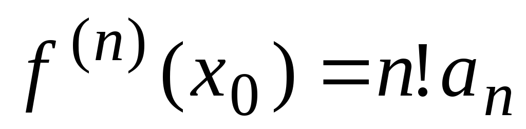
, where

So, the coefficients are found

,
,
, …,
,….,

substituting which into the series (*), we get

The resulting series is called next to Taylor for function
.

Thus, we have established that if the function can be expanded into a power series in powers (x - x 0 ), then this expansion is unique and the resulting series is necessarily a Taylor series.

Note that the Taylor series can be obtained for any function that has derivatives of any order at the point x = x 0 . But this does not mean that an equal sign can be placed between the function and the resulting series, i.e. that the sum of the series is equal to the original function. Firstly, such an equality can only make sense in the region of convergence, and the Taylor series obtained for the function may diverge, and secondly, if the Taylor series converges, then its sum may not coincide with the original function.

3.2. Sufficient conditions for the decomposability of a function in a Taylor series

Let us formulate a statement with the help of which the task will be solved.

If the function
in some neighborhood of point x 0 has derivatives up to (n+ 1) of order inclusive, then in this neighborhood we haveformula Taylor

WhereR n (X)-the remainder term of the Taylor formula – has the form (Lagrange form)

Where dotξ lies between x and x 0 .

Note that there is a difference between the Taylor series and the Taylor formula: the Taylor formula is a finite sum, i.e. P - fixed number.

Recall that the sum of the series S(x) can be defined as the limit of a functional sequence of partial sums S P (x) at some interval X:

.

According to this, to expand a function into a Taylor series means to find a series such that for any XX

Let us write Taylor's formula in the form where

notice, that
defines the error we get, replace the function f(x) polynomial S n (x).

If
, That
,those. the function is expanded into a Taylor series. Vice versa, if
, That
.

Thus we proved criterion for the decomposability of a function in a Taylor series.

In order for the functionf(x) expands into a Taylor series, it is necessary and sufficient that on this interval
, WhereR n (x) is the remainder term of the Taylor series.

Using the formulated criterion, one can obtain sufficientconditions for the decomposability of a function in a Taylor series.

If insome neighborhood of the point x 0 the absolute values ​​of all derivatives of the function are limited to the same number M≥ 0, i.e.

, To in this neighborhood the function expands into a Taylor series.

From the above it follows algorithmfunction expansion f(x) in the Taylor series in the vicinity of a point X 0 :

1. Finding derivatives of functions f(x):

f(x), f’(x), f”(x), f’”(x), f (n) (x),…

2. Calculate the value of the function and the values ​​of its derivatives at the point X 0

f(x 0 ), f’(x 0 ), f”(x 0 ), f’”(x 0 ), f (n) (x 0 ),…

3. We formally write the Taylor series and find the region of convergence of the resulting power series.

4. We check the fulfillment of sufficient conditions, i.e. we establish for which X from the convergence region, remainder term R n (x) tends to zero as
or
.

The expansion of functions into a Taylor series using this algorithm is called expansion of a function into a Taylor series by definition or direct decomposition.

If the function f(x) has derivatives of all orders on a certain interval containing point a, then the Taylor formula can be applied to it:
,
Where r n– the so-called remainder term or remainder of the series, it can be estimated using the Lagrange formula:
, where the number x is between x and a.

f(x)=

at point x 0 = Number of row elements 3 4 5 6 7

Use the expansion of elementary functions e x , cos(x), sin(x), ln(1+x), (1+x) m

Rules for entering functions:

If for some value X r n→0 at n→∞, then in the limit the Taylor formula becomes convergent for this value Taylor series:
,
Thus, the function f(x) can be expanded into a Taylor series at the point x under consideration if:
1) it has derivatives of all orders;
2) the constructed series converges at this point.

When a = 0 we get a series called near Maclaurin:
,
Expansion of the simplest (elementary) functions in the Maclaurin series:
Exponential functions
, R=∞
Trigonometric functions
, R=∞
, R=∞
, (-π/2< x < π/2), R=π/2
The function actgx does not expand in powers of x, because ctg0=∞
Hyperbolic functions


Logarithmic functions
, -1
Binomial series
.

Example No. 1. Expand the function into a power series f(x)= 2x.
Solution. Let us find the values ​​of the function and its derivatives at X=0
f(x) = 2x, f( 0) = 2 0 =1;
f"(x) = 2x ln2, f"( 0) = 2 0 ln2= ln2;
f""(x) = 2x ln 2 2, f""( 0) = 2 0 ln 2 2= ln 2 2;
…
f(n)(x) = 2x ln n 2, f(n)( 0) = 2 0 ln n 2=ln n 2.
Substituting the obtained values ​​of the derivatives into the Taylor series formula, we obtain:

The radius of convergence of this series is equal to infinity, therefore this expansion is valid for -∞<x<+∞.

Example No. 2. Write the Taylor series in powers ( X+4) for function f(x)= e x.
Solution. Finding the derivatives of the function e x and their values ​​at the point X=-4.
f(x)= e x, f(-4) = e -4 ;
f"(x)= e x, f"(-4) = e -4 ;
f""(x)= e x, f""(-4) = e -4 ;
…
f(n)(x)= e x, f(n)( -4) = e -4 .
Therefore, the required Taylor series of the function has the form:

This expansion is also valid for -∞<x<+∞.

Example No. 3. Expand a function f(x)=ln x in a series in powers ( X- 1),
(i.e. in the Taylor series in the vicinity of the point X=1).
Solution. Find the derivatives of this function.
f(x)=lnx , , , ,

f(1)=ln1=0, f"(1)=1, f""(1)=-1, f"""(1)=1*2,..., f (n) =(- 1) n-1 (n-1)!
Substituting these values ​​into the formula, we obtain the desired Taylor series:

Using d'Alembert's test, you can verify that the series converges at ½x-1½<1 . Действительно,

The series converges if ½ X- 1½<1, т.е. при 0<x<2. При X=2 we obtain an alternating series that satisfies the conditions of the Leibniz criterion. When x=0 the function is not defined. Thus, the region of convergence of the Taylor series is the half-open interval (0;2].

Example No. 4. Expand the function into a power series.
Solution. In expansion (1) we replace x with -x 2, we get:
, -∞

Example No. 5. Expand the function into a Maclaurin series.
Solution. We have
Using formula (4), we can write:

substituting –x instead of x in the formula, we get:

From here we find: ln(1+x)-ln(1-x) = -
Opening the brackets, rearranging the terms of the series and bringing similar terms, we get
. This series converges in the interval (-1;1), since it is obtained from two series, each of which converges in this interval.

Comment .
Formulas (1)-(5) can also be used to expand the corresponding functions into a Taylor series, i.e. for expanding functions in positive integer powers ( Ha). To do this, it is necessary to perform such identical transformations on a given function in order to obtain one of the functions (1)-(5), in which instead X costs k( Ha) m , where k is a constant number, m is a positive integer. It is often convenient to make a change of variable t=Ha and expand the resulting function with respect to t in the Maclaurin series.

This method is based on the theorem on the uniqueness of the expansion of a function in a power series. The essence of this theorem is that in the neighborhood of the same point two different power series cannot be obtained that would converge to the same function, no matter how its expansion is performed.

Example No. 5a. Expand the function in a Maclaurin series and indicate the region of convergence.
Solution. First we find 1-x-6x 2 =(1-3x)(1+2x) , .
to elementary:

The fraction 3/(1-3x) can be considered as the sum of an infinitely decreasing geometric progression with a denominator of 3x, if |3x|< 1. Аналогично, дробь 2/(1+2x) как сумму бесконечно убывающей геометрической прогрессии знаменателем -2x, если |-2x| < 1. В результате получим разложение в степенной ряд

with convergence region |x|< 1/3.

Example No. 6. Expand the function into a Taylor series in the vicinity of the point x = 3.
Solution. This problem can be solved, as before, using the definition of the Taylor series, for which we need to find the derivatives of the function and their values ​​at X=3. However, it will be easier to use the existing expansion (5):
=
The resulting series converges at or –3

Example No. 7. Write the Taylor series in powers (x -1) of the function ln(x+2) .
Solution.


The series converges at , or -2< x < 5.

Example No. 8. Expand the function f(x)=sin(πx/4) into a Taylor series in the vicinity of the point x =2.
Solution. Let's make the replacement t=x-2:

Using expansion (3), in which we substitute π / 4 t in place of x, we obtain:

The resulting series converges to the given function at -∞< π / 4 t<+∞, т.е. при (-∞Thus,
, (-∞

Approximate calculations using power series

Power series are widely used in approximate calculations. With their help, you can calculate the values ​​of roots, trigonometric functions, logarithms of numbers, and definite integrals with a given accuracy. Series are also used when integrating differential equations.
Consider the expansion of a function in a power series:

In order to calculate the approximate value of a function at a given point X, belonging to the region of convergence of the indicated series, the first ones are left in its expansion n members ( n– a finite number), and the remaining terms are discarded:

To estimate the error of the obtained approximate value, it is necessary to estimate the discarded remainder rn (x) . To do this, use the following techniques:

• if the resulting series is alternating, then the following property is used: for an alternating series that satisfies the Leibniz conditions, the remainder of the series in absolute value does not exceed the first discarded term.
• if a given series is of constant sign, then the series composed of discarded terms is compared with an infinitely decreasing geometric progression.
• in the general case, to estimate the remainder of the Taylor series, you can use the Lagrange formula: a x ).

Example No. 1. Calculate ln(3) to the nearest 0.01.
Solution. Let's use the expansion where x=1/2 (see example 5 in the previous topic):

Let's check whether we can discard the remainder after the first three terms of the expansion; to do this, we will evaluate it using the sum of an infinitely decreasing geometric progression:

So we can discard this remainder and get

Example No. 2. Calculate to the nearest 0.0001.
Solution. Let's use the binomial series. Since 5 3 is the cube of an integer closest to 130, it is advisable to represent the number 130 as 130 = 5 3 +5.



since already the fourth term of the resulting alternating series satisfying the Leibniz criterion is less than the required accuracy:
, so it and the terms following it can be discarded.
Many practically necessary definite or improper integrals cannot be calculated using the Newton-Leibniz formula, because its application is associated with finding the antiderivative, which often does not have an expression in elementary functions. It also happens that finding an antiderivative is possible, but it is unnecessarily labor-intensive. However, if the integrand function is expanded into a power series, and the limits of integration belong to the interval of convergence of this series, then an approximate calculation of the integral with a predetermined accuracy is possible.

Example No. 3. Calculate the integral ∫ 0 1 4 sin (x) x to within 10 -5 .
Solution. The corresponding indefinite integral cannot be expressed in elementary functions, i.e. represents a “non-permanent integral”. The Newton-Leibniz formula cannot be applied here. Let's calculate the integral approximately.
Dividing term by term the series for sin x on x, we get:

Integrating this series term by term (this is possible, since the limits of integration belong to the interval of convergence of this series), we obtain:

Since the resulting series satisfies Leibniz’s conditions and it is enough to take the sum of the first two terms to obtain the desired value with a given accuracy.
Thus, we find
.

Example No. 4. Calculate the integral ∫ 0 1 4 e x 2 with an accuracy of 0.001.
Solution.
. Let's check whether we can discard the remainder after the second term of the resulting series.
0.0001<0.001. Следовательно, .

"Find the Maclaurin series expansion of the function f(x)"- this is exactly what the task in higher mathematics sounds like, which some students can do, while others cannot cope with the examples. There are several ways to expand a series in powers; here we will give a technique for expanding functions into a Maclaurin series. When developing a function in a series, you need to be good at calculating derivatives.

Example 4.7 Expand a function in powers of x

Calculations: We perform the expansion of the function according to the Maclaurin formula. First, let's expand the denominator of the function into a series

Finally, multiply the expansion by the numerator.
The first term is the value of the function at zero f (0) = 1/3.
Let's find the derivatives of the function of the first and higher orders f (x) and the value of these derivatives at the point x=0




Next, based on the pattern of changes in the value of derivatives at 0, we write the formula for the nth derivative

So, we represent the denominator in the form of an expansion in the Maclaurin series

We multiply by the numerator and obtain the desired expansion of the function in a series in powers of x

As you can see, there is nothing complicated here.
All key points are based on the ability to calculate derivatives and quickly generalize the value of the higher order derivative at zero. The following examples will help you learn how to quickly arrange a function in a series.

Example 4.10 Find the Maclaurin series expansion of the function

Calculations: As you may have guessed, we will put the cosine in the numerator in a series. To do this, you can use formulas for infinitesimal quantities, or derive the cosine expansion through derivatives. As a result, we arrive at the following series in powers of x

As you can see, we have a minimum of calculations and a compact representation of the series expansion.

Example 4.16 Expand a function in powers of x:
7/(12-x-x^2)
Calculations: In this kind of examples, it is necessary to expand the fraction through the sum of simple fractions.
We will not show how to do this now, but with the help of indefinite coefficients we will arrive at the sum of fractions.
Next we write the denominators in exponential form

It remains to expand the terms using the Maclaurin formula. Summing up the terms at the same powers of “x”, we compose a formula for the general term of the expansion of a function in a series



The last part of the transition to the series at the beginning is difficult to implement, since it is difficult to combine the formulas for paired and unpaired indices (degrees), but with practice you will get better at it.

Example 4.18 Find the Maclaurin series expansion of the function

Calculations: Let's find the derivative of this function:

Let's expand the function into a series using one of McLaren's formulas:

We sum the series term by term based on the fact that both are absolutely identical. Having integrated the entire series term by term, we obtain the expansion of the function into a series in powers of x

There is a transition between the last two lines of the expansion which will take a lot of your time at the beginning. Generalizing a series formula isn't easy for everyone, so don't worry about not being able to get a nice, compact formula.

Example 4.28 Find the Maclaurin series expansion of the function:

Let's write the logarithm as follows

Using Maclaurin’s formula, we expand the logarithm function in a series in powers of x

The final convolution is complex at first glance, but when alternating signs you will always get something similar. Input lesson on the topic of scheduling functions in a row is completed. Other equally interesting decomposition schemes will be discussed in detail in the following materials.