Solution using the Gaussian method. Gaussian method (sequential elimination of unknowns)
Educational institution "Belarusian State
Agricultural Academy"
Department higher mathematics
to study the topic “Gauss method for solving systems of linear
equations" by students of the accounting faculty of correspondence education (NISPO)
Gorki, 2013
Gauss method for solving systems linear equations
Equivalent systems of equations
Two systems of linear equations are said to be equivalent if each solution of one of them is a solution of the other. The process of solving a system of linear equations consists of sequentially transforming it into an equivalent system using the so-called elementary transformations , which are:
1) rearrangement of any two equations of the system;
2) multiplying both sides of any equation of the system by a nonzero number;
3) adding to any equation another equation multiplied by any number;
4) crossing out an equation consisting of zeros, i.e. equations of the form
Gaussian elimination
Consider the system m linear equations with n unknown:

The essence of the Gauss method or method sequential elimination the unknowns are as follows.
First, using elementary transformations, the unknown is eliminated from all equations of the system except the first. Such system transformations are called Gaussian elimination step . The unknown is called enabling variable at the first step of transformation. The coefficient is called resolution factor , the first equation is called resolving equation , and the column of coefficients at permission column .
When performing one step of Gaussian elimination, you need to use the following rules:
1) the coefficients and the free term of the resolving equation remain unchanged;
2) the coefficients of the resolution column located below the resolution coefficient become zero;
3) all other coefficients and free terms when performing the first step are calculated according to the rectangle rule:
 , Where i=2,3,…,m; j=2,3,…,n.
We will perform similar transformations on the second equation of the system. This will lead to a system in which the unknown will be eliminated in all equations except the first two. As a result of such transformations over each of the equations of the system (direct progression of the Gauss method), the original system is reduced to an equivalent step system of one of the following types.
Reverse Gaussian method
Step system

has a triangular appearance and that's it  (i=1,2,…,n). Such a system has only decision. The unknowns are determined starting from the last equation (reverse of the Gaussian method).
The step system has the form

where, i.e. the number of equations of the system is less than or equal to the number of unknowns. This system has no solutions, since the last equation will not be satisfied for any values of the variable.
Step type system

has countless solutions. From the last equation, the unknown is expressed through the unknowns  . Then, in the penultimate equation, instead of the unknown, its expression is substituted through the unknowns . Continuing the reverse of the Gaussian method, the unknowns
  can be expressed in terms of unknowns . In this case, the unknowns are called free
and can take any values, and unknown
can be expressed in terms of unknowns . In this case, the unknowns are called free
and can take any values, and unknown  basic.
When solving systems in practice, it is convenient to perform all transformations not with a system of equations, but with an extended matrix of the system, consisting of coefficients for unknowns and a column of free terms.
Example 1. Solve system of equations 
Solution. Let's create an extended matrix of the system and perform elementary transformations:


 .
.
In the extended matrix of the system, the number 3 (it is highlighted) is the resolution coefficient, the first row is the resolution row, and the first column is the resolution column. When moving to the next matrix, the resolution row does not change; all elements of the resolution column below the resolution element are replaced by zeros. And all other elements of the matrix are recalculated according to the quadrilateral rule. Instead of element 4 in the second line we write  , instead of element -3 in the second line it will be written
 ![]() etc. Thus, the second matrix will be obtained. The resolution element of this matrix will be the number 18 in the second row. To form the next (third matrix), we leave the second row unchanged, in the column under the resolving element we write zero and recalculate the remaining two elements: instead of the number 1 we write
etc. Thus, the second matrix will be obtained. The resolution element of this matrix will be the number 18 in the second row. To form the next (third matrix), we leave the second row unchanged, in the column under the resolving element we write zero and recalculate the remaining two elements: instead of the number 1 we write  , and instead of the number 16 we write .
As a result, the original system was reduced to an equivalent system

From the third equation we find ![]() . Let's substitute this value into the second equation:
. Let's substitute this value into the second equation:  y=3. Let’s substitute the found values into the first equation y And z:
 ![]() , x=2.
, x=2.
Thus, the solution to this system of equations is x=2, y=3, ![]() .
.
Example 2. Solve system of equations 
Solution. Let us perform elementary transformations on the extended matrix of the system:


In the second matrix, each element of the third row is divided by 2.


In the fourth matrix, each element of the third and fourth rows was divided by 11.
 . The resulting matrix corresponds to the system of equations
Deciding this system, let's find  ,
,  , .
, .
Example 3. Solve system of equations

Solution. Let's write the extended matrix of the system and perform elementary transformations:


 .
.
In the second matrix, each element of the second, third and fourth rows was divided by 7.
As a result, a system of equations was obtained

equivalent to the original one.
Since there are two fewer equations than unknowns, then from the second equation  . Let's substitute the expression for into the first equation: ,
  .
.
Thus, the formulas  give a general solution to this system of equations. Unknowns are free and can take any value.
Let, for example,  Then
Then  And
And  . Solution


 is one of the particular solutions of the system, of which there are countless.
Questions for self-control of knowledge
1) What transformations of linear systems are called elementary?
2) What transformations of the system are called the Gaussian elimination step?
3) What is a resolving variable, resolving coefficient, resolving column?
4) What rules should be used when performing one step of Gaussian elimination?
Let the system be given, ∆≠0. (1)Gauss method is a method of sequentially eliminating unknowns.
The essence of the Gauss method is to transform (1) to a system with a triangular matrix, from which the values of all unknowns are then obtained sequentially (in reverse). Let's consider one of the computational schemes. This circuit is called a single division circuit. So let's look at this diagram. Let a 11 ≠0 (leading element) divide the first equation by a 11. We get
(2)
Using equation (2), it is easy to eliminate the unknowns x 1 from the remaining equations of the system (to do this, it is enough to subtract equation (2) from each equation, previously multiplied by the corresponding coefficient for x 1), that is, in the first step we obtain
.
In other words, at step 1, each element of subsequent rows, starting from the second, is equal to the difference between the original element and the product of its “projection” onto the first column and the first (transformed) row.
Following this, leaving the first equation alone, we perform a similar transformation over the remaining equations of the system obtained in the first step: we select from among them the equation with the leading element and, with its help, exclude x 2 from the remaining equations (step 2).
After n steps, instead of (1), we obtain an equivalent system  (3)
(3)
Thus, at the first stage we obtain a triangular system (3). This stage is called forward stroke.
At the second stage (reverse), we find sequentially from (3) the values x n, x n -1, ..., x 1.
Let us denote the resulting solution as x 0 . Then the difference ε=b-A x 0 called residual.
If ε=0, then the found solution x 0 is correct.
Calculations using the Gaussian method are performed in two stages:
- The first stage is called the forward method. At the first stage, the original system is converted to a triangular form.
- The second stage is called the reverse stroke. At the second stage, a triangular system equivalent to the original one is solved.
At each step, the leading element was assumed to be nonzero. If this is not the case, then any other element can be used as a leading element, as if rearranging the equations of the system.
Purpose of the Gauss method
The Gauss method is designed for solving systems of linear equations. Refers to direct solution methods.Types of Gaussian method
- Classical Gaussian method;
- Modifications of the Gauss method. One of the modifications of the Gaussian method is a scheme with the choice of the main element. A feature of the Gauss method with the choice of the main element is such a rearrangement of the equations so that at the kth step the leading element turns out to be the largest element in the kth column.
- Jordano-Gauss method;
Let's illustrate the difference Jordano-Gauss method from the Gaussian method with examples.
Example of a solution using the Gaussian method
Let's solve the system: 
For ease of calculation, let's swap the lines: 
Let's multiply the 2nd line by (2). Add the 3rd line to the 2nd 
Multiply the 2nd line by (-1). Add the 2nd line to the 1st 
From the 1st line we express x 3:
From the 2nd line we express x 2:
From the 3rd line we express x 1:
An example of a solution using the Jordano-Gauss method
Let us solve the same SLAE using the Jordano-Gauss method. 
We will sequentially select the resolving element RE, which lies on the main diagonal of the matrix.
The resolution element is equal to (1).
NE = SE - (A*B)/RE
RE - resolving element (1), A and B - matrix elements forming a rectangle with elements STE and RE.
Let's present the calculation of each element in the form of a table:
| x 1 | x 2 | x 3 | B |
| 1 / 1 = 1 | 2 / 1 = 2 | -2 / 1 = -2 | 1 / 1 = 1 |

The resolving element is equal to (3).
In place of the resolving element we get 1, and in the column itself we write zeros.
All other elements of the matrix, including elements of column B, are determined by the rectangle rule.
To do this, we select four numbers that are located at the vertices of the rectangle and always include the resolving element RE.
| x 1 | x 2 | x 3 | B |
| 0 / 3 = 0 | 3 / 3 = 1 | 1 / 3 = 0.33 | 4 / 3 = 1.33 |

The resolution element is (-4).
In place of the resolving element we get 1, and in the column itself we write zeros.
All other elements of the matrix, including elements of column B, are determined by the rectangle rule.
To do this, we select four numbers that are located at the vertices of the rectangle and always include the resolving element RE.
Let's present the calculation of each element in the form of a table:
| x 1 | x 2 | x 3 | B |
| 0 / -4 = 0 | 0 / -4 = 0 | -4 / -4 = 1 | -4 / -4 = 1 |
Answer: x 1 = 1, x 2 = 1, x 3 = 1
Implementation of the Gaussian method
The Gaussian method is implemented in many programming languages, in particular: Pascal, C++, php, Delphi, and there is also an online implementation of the Gaussian method.Using the Gaussian Method
Application of the Gauss method in game theory
In game theory, when finding the maximin optimal strategy of a player, a system of equations is compiled, which is solved by the Gaussian method.Application of the Gauss method in solving differential equations
To find a partial solution to a differential equation, first find derivatives of the appropriate degree for the written partial solution (y=f(A,B,C,D)), which are substituted into the original equation. Next to find variables A,B,C,D a system of equations is compiled and solved by the Gaussian method.Application of the Jordano-Gauss method in linear programming
IN linear programming, in particular, in the simplex method, the rectangle rule, which uses the Jordano-Gauss method, is used to transform the simplex table at each iteration.One of the simplest ways to solve a system of linear equations is a technique based on the calculation of determinants ( Cramer's rule). Its advantage is that it allows you to immediately record the solution; it is especially convenient in cases where the coefficients of the system are not numbers, but some parameters. Its disadvantage is the cumbersomeness of calculations in the case large number equations; moreover, Cramer's rule is not directly applicable to systems in which the number of equations does not coincide with the number of unknowns. In such cases, it is usually used Gaussian method.
Systems of linear equations having the same set of solutions are called equivalent. Obviously, many solutions linear system does not change if any equations are swapped, or if one of the equations is multiplied by some non-zero number, or if one equation is added to another.
Gauss method (method of sequential elimination of unknowns) is that with the help of elementary transformations the system is reduced to an equivalent system of a step type. First, using the 1st equation, we eliminate x 1 of all subsequent equations of the system. Then, using the 2nd equation, we eliminate x 2 from the 3rd and all subsequent equations. This process, called direct Gaussian method, continues until there is only one unknown left on the left side of the last equation x n. After this it is done inverse of the Gaussian method– solving the last equation, we find x n; after that, using this value, from the penultimate equation we calculate x n–1, etc. We find the last one x 1 from the first equation.
It is convenient to carry out Gaussian transformations by performing transformations not with the equations themselves, but with the matrices of their coefficients. Consider the matrix:
called extended matrix of the system, because, in addition to the main matrix of the system, it includes a column of free terms. The Gaussian method is based on reducing the main matrix of the system to a triangular form (or trapezoidal form in the case of non-square systems) using elementary row transformations (!) of the extended matrix of the system.
Example 5.1. Solve the system using the Gaussian method:

Solution. Let's write out the extended matrix of the system and, using the first row, after that we will reset the remaining elements:
 we get zeros in the 2nd, 3rd and 4th rows of the first column:


Now we need all elements in the second column below the 2nd row to be equal to zero. To do this, you can multiply the second line by –4/7 and add it to the 3rd line. However, in order not to deal with fractions, let's create a unit in the 2nd row of the second column and only
Now, to get a triangular matrix, you need to reset the element of the fourth row of the 3rd column; to do this, you can multiply the third row by 8/54 and add it to the fourth. However, in order not to deal with fractions, we will swap the 3rd and 4th rows and the 3rd and 4th columns and only after that we will reset the specified element. Note that when rearranging the columns, the corresponding variables change places and this must be remembered; other elementary transformations with columns (addition and multiplication by a number) cannot be performed!

The last simplified matrix corresponds to a system of equations equivalent to the original one:

From here, using the inverse of the Gaussian method, we find from the fourth equation x 3 = –1; from the third x 4 = –2, from the second x 2 = 2 and from the first equation x 1 = 1. In matrix form, the answer is written as
We considered the case when the system is definite, i.e. when there is only one solution. Let's see what happens if the system is inconsistent or uncertain.
Example 5.2. Explore the system using the Gaussian method:

Solution. We write out and transform the extended matrix of the system

We write a simplified system of equations:

Here, in the last equation it turns out that 0=4, i.e. contradiction. Consequently, the system has no solution, i.e. she incompatible. à
Example 5.3. Explore and solve the system using the Gaussian method:

Solution. We write out and transform the extended matrix of the system:

As a result of the transformations, the last line contains only zeros. This means that the number of equations has decreased by one:

Thus, after simplifications, there are two equations left, and four unknowns, i.e. two unknown "extra". Let them be "superfluous", or, as they say, free variables, will x 3 and x 4 . Then

Believing x 3 = 2a And x 4 = b, we get x 2 = 1–a And x 1 = 2b–a; or in matrix form
A solution written in this way is called general, because, giving parameters a And b different meanings, everything can be described possible solutions systems. a
Gauss method perfect for solving systems of linear algebraic equations (SLAEs). It has a number of advantages compared to other methods:
- firstly, there is no need to first examine the system of equations for consistency;
- secondly, the Gauss method can solve not only SLAEs in which the number of equations coincides with the number of unknown variables and the main matrix of the system is non-singular, but also systems of equations in which the number of equations does not coincide with the number of unknown variables or the determinant of the main matrix is equal to zero;
- thirdly, the Gaussian method leads to results with a relatively small number of computational operations.
Brief overview of the article.
First let's give necessary definitions and introduce the notation.
Next, we will describe the algorithm of the Gauss method for the simplest case, that is, for systems of linear algebraic equations, the number of equations in which coincides with the number of unknown variables and the determinant of the main matrix of the system is not equal to zero. When solving such systems of equations, the essence of the Gauss method is most clearly visible, which is the sequential elimination of unknown variables. Therefore, the Gaussian method is also called the method of sequential elimination of unknowns. We will show detailed solutions of several examples.
In conclusion, we will consider the solution by the Gauss method of systems of linear algebraic equations, the main matrix of which is either rectangular or singular. The solution to such systems has some features, which we will examine in detail using examples.
Page navigation.
Basic definitions and notations.
Consider a system of p linear equations with n unknowns (p can be equal to n):
Where are unknown variables, are numbers (real or complex), and are free terms.
If ![]() , then the system of linear algebraic equations is called homogeneous, otherwise - heterogeneous.
, then the system of linear algebraic equations is called homogeneous, otherwise - heterogeneous.
The set of values of unknown variables for which all equations of the system become identities is called decision of the SLAU.
If there is at least one solution to a system of linear algebraic equations, then it is called joint, otherwise - non-joint.
If a SLAE has a unique solution, then it is called certain. If there is more than one solution, then the system is called uncertain.
They say that the system is written in coordinate form, if it has the form
.
This system in matrix form records has the form , where  - the main matrix of the SLAE, - the matrix of the column of unknown variables, - the matrix of free terms.
If we add a matrix-column of free terms to matrix A as the (n+1)th column, we get the so-called extended matrix systems of linear equations. Typically, an extended matrix is denoted by the letter T, and the column of free terms is separated by a vertical line from the remaining columns, that is, 
The square matrix A is called degenerate, if its determinant is zero. If , then matrix A is called non-degenerate.
The following point should be noted.
If you perform the following actions with a system of linear algebraic equations
- swap two equations,
- multiply both sides of any equation by an arbitrary and non-zero real (or complex) number k,
- to both sides of any equation add the corresponding parts of another equation, multiplied by an arbitrary number k,
then you get an equivalent system that has the same solutions (or, just like the original one, has no solutions).
For an extended matrix of a system of linear algebraic equations, these actions will mean carrying out elementary transformations with the rows:
- swapping two lines,
- multiplying all elements of any row of matrix T by a nonzero number k,
- adding to the elements of any row of a matrix the corresponding elements of another row, multiplied by an arbitrary number k.
Now we can proceed to the description of the Gauss method.
Solving systems of linear algebraic equations, in which the number of equations is equal to the number of unknowns and the main matrix of the system is non-singular, using the Gauss method.
What would we do at school if we were given the task of finding a solution to a system of equations?  .
.
Some would do that.
Note that adding to the left side of the second equation left side first, and to the right side - the right one, you can get rid of the unknown variables x 2 and x 3 and immediately find x 1: 
We substitute the found value x 1 =1 into the first and third equations of the system: 
If we multiply both sides of the third equation of the system by -1 and add them to the corresponding parts of the first equation, we get rid of the unknown variable x 3 and can find x 2: 
We substitute the resulting value x 2 = 2 into the third equation and find the remaining unknown variable x 3: 
Others would have done differently.
Let us resolve the first equation of the system with respect to the unknown variable x 1 and substitute the resulting expression into the second and third equations of the system in order to exclude this variable from them: 
Now let’s solve the second equation of the system for x 2 and substitute the result obtained into the third equation to eliminate the unknown variable x 2 from it: 
From the third equation of the system it is clear that x 3 =3. From the second equation we find ![]() , and from the first equation we get .
, and from the first equation we get .
Familiar solutions, right?
The most interesting thing here is that the second solution method is essentially the method of sequential elimination of unknowns, that is, the Gaussian method. When we expressed the unknown variables (first x 1, on next stage x 2 ) and substituted them into the remaining equations of the system, thereby eliminating them. We carried out elimination until there was only one unknown variable left in the last equation. The process of sequentially eliminating unknowns is called direct Gaussian method. After completing the forward move, we have the opportunity to calculate the unknown variable found in the last equation. With its help, we find the next unknown variable from the penultimate equation, and so on. The process of sequentially finding unknown variables while moving from the last equation to the first is called inverse of the Gaussian method.
It should be noted that when we express x 1 in terms of x 2 and x 3 in the first equation, and then substitute the resulting expression into the second and third equations, the following actions lead to the same result:
Indeed, such a procedure also makes it possible to eliminate the unknown variable x 1 from the second and third equations of the system: 
Nuances with the elimination of unknown variables using the Gaussian method arise when the equations of the system do not contain some variables.
For example, in SLAU  in the first equation there is no unknown variable x 1 (in other words, the coefficient in front of it is zero). Therefore, we cannot solve the first equation of the system for x 1 in order to eliminate this unknown variable from the remaining equations. The way out of this situation is to swap the equations of the system. Since we are considering systems of linear equations whose determinants of the main matrices are different from zero, there is always an equation in which the variable we need is present, and we can rearrange this equation to the position we need. For our example, it is enough to swap the first and second equations of the system
  , then you can resolve the first equation for x 1 and exclude it from the remaining equations of the system (although x 1 is no longer present in the second equation).
We hope you get the gist.
Let's describe Gaussian method algorithm.
Suppose we need to solve a system of n linear algebraic equations with n unknowns variables of the form  , and let the determinant of its main matrix be different from zero.
We will assume that , since we can always achieve this by rearranging the equations of the system. Let's eliminate the unknown variable x 1 from all equations of the system, starting with the second. To do this, to the second equation of the system we add the first, multiplied by , to the third equation we add the first, multiplied by , and so on, to the nth equation we add the first, multiplied by . The system of equations after such transformations will take the form 
where and  .
.
We would have arrived at the same result if we had expressed x 1 in terms of other unknown variables in the first equation of the system and substituted the resulting expression into all other equations. Thus, the variable x 1 is excluded from all equations, starting from the second.
Next, we proceed in a similar way, but only with part of the resulting system, which is marked in the figure 
To do this, to the third equation of the system we add the second, multiplied by , to the fourth equation we add the second, multiplied by , and so on, to the nth equation we add the second, multiplied by . The system of equations after such transformations will take the form 
where and  . Thus, the variable x 2 is excluded from all equations, starting from the third.
Next, we proceed to eliminating the unknown x 3, while we act similarly with the part of the system marked in the figure 
So we continue the direct progression of the Gaussian method until the system takes the form 
From this moment we begin the reverse of the Gaussian method: we calculate x n from the last equation as , using the obtained value of x n we find x n-1 from the penultimate equation, and so on, we find x 1 from the first equation.
Let's look at the algorithm using an example.
Example.
 Gauss method.
Solution.
The coefficient a 11 is different from zero, so let’s proceed to the direct progression of the Gaussian method, that is, to the exclusion of the unknown variable x 1 from all equations of the system except the first. To do this, to the left and right sides of the second, third and fourth equations, add the left and right sides of the first equation, multiplied by , respectively.  And :
And : 
The unknown variable x 1 has been eliminated, let's move on to eliminating x 2 . To the left and right sides of the third and fourth equations of the system we add the left and right sides of the second equation, multiplied by respectively  And
And  :
:
To complete the forward progression of the Gaussian method, we need to eliminate the unknown variable x 3 from the last equation of the system. Let us add to the left and right sides of the fourth equation, respectively, the left and right sides of the third equation, multiplied by  :
:
You can begin the reverse of the Gaussian method.
From the last equation we have  ,
,
from the third equation we get,
from the second,
from the first one.
To check, you can substitute the obtained values of the unknown variables into the original system of equations. All equations turn into identities, which indicates that the solution using the Gauss method was found correctly.
Answer:
Now let’s give a solution to the same example using the Gaussian method in matrix notation.
Example.
Find the solution to the system of equations Gauss method.
Solution.
The extended matrix of the system has the form  . At the top of each column are the unknown variables that correspond to the elements of the matrix.
The direct approach of the Gaussian method here involves reducing the extended matrix of the system to a trapezoidal form using elementary transformations. This process is similar to the elimination of unknown variables that we did with the system in coordinate form. Now you will see this.
Let's transform the matrix so that all elements in the first column, starting from the second, become zero. To do this, to the elements of the second, third and fourth lines we add the corresponding elements of the first line multiplied by , and accordingly: 
Next, we transform the resulting matrix so that in the second column all elements, starting from the third, become zero. This would correspond to eliminating the unknown variable x 2 . To do this, to the elements of the third and fourth rows we add the corresponding elements of the first row of the matrix, multiplied by respectively And :

It remains to exclude the unknown variable x 3 from the last equation of the system. To do this, to the elements of the last row of the resulting matrix we add the corresponding elements of the penultimate row, multiplied by :

It should be noted that this matrix corresponds to a system of linear equations 
which was obtained earlier after a forward move.
It's time to turn back. In matrix notation, the inverse of the Gaussian method involves transforming the resulting matrix such that the matrix marked in the figure 
became diagonal, that is, took the form 
where are some numbers.
These transformations are similar to the forward transformations of the Gaussian method, but are performed not from the first line to the last, but from the last to the first.
Add to the elements of the third, second and first lines the corresponding elements of the last line, multiplied by  , on and on
  respectively:
Now add to the elements of the second and first lines the corresponding elements of the third line, multiplied by and by, respectively: 
At the last step of the reverse Gaussian method, to the elements of the first row we add the corresponding elements of the second row, multiplied by: 
The resulting matrix corresponds to the system of equations  , from where we find the unknown variables.
Answer:
NOTE.
When using the Gauss method to solve systems of linear algebraic equations, approximate calculations should be avoided, as this can lead to completely incorrect results. We recommend not rounding decimals. Better from decimals go to ordinary fractions.
Example.
Solve a system of three equations using the Gauss method  .
.
Solution.
Note that in this example the unknown variables have a different designation (not x 1, x 2, x 3, but x, y, z). Let's move on to ordinary fractions: 
Let us exclude the unknown x from the second and third equations of the system: 
In the resulting system, the unknown variable y is absent in the second equation, but y is present in the third equation, therefore, let’s swap the second and third equations: 
This completes the direct progression of the Gauss method (there is no need to exclude y from the third equation, since this unknown variable no longer exists).
Let's start the reverse move.
From the last equation we find  ,
,
from the penultimate 
from the first equation we have 
Answer:
X = 10, y = 5, z = -20.
Solving systems of linear algebraic equations in which the number of equations does not coincide with the number of unknowns or the main matrix of the system is singular, using the Gauss method.
Systems of equations, the main matrix of which is rectangular or square singular, may have no solutions, may have a single solution, or may have an infinite number of solutions.
Now we will understand how the Gauss method allows us to establish the compatibility or inconsistency of a system of linear equations, and in the case of its compatibility, determine all solutions (or one single solution).
In principle, the process of eliminating unknown variables in the case of such SLAEs remains the same. However, it is worth going into detail about some situations that may arise.
Let's move on to the most important stage.
So, let us assume that the system of linear algebraic equations, after completing the forward progression of the Gauss method, takes the form  and not a single equation was reduced to (in this case we would conclude that the system is incompatible). A logical question arises: “What to do next”?
Let us write down the unknown variables that come first in all equations of the resulting system: 
In our example these are x 1, x 4 and x 5. On the left sides of the equations of the system we leave only those terms that contain the written unknown variables x 1, x 4 and x 5, the remaining terms are transferred to the right side of the equations with the opposite sign: 
Let's give the unknown variables that are on the right sides of the equations arbitrary values, where ![]() - arbitrary numbers:
- arbitrary numbers: 
After this, the right-hand sides of all equations of our SLAE contain numbers and we can proceed to the reverse of the Gaussian method.
From the last equation of the system we have, from the penultimate equation we find, from the first equation we get 
The solution to a system of equations is a set of values of unknown variables 
Giving Numbers ![]() different values we will get various solutions systems of equations. That is, our system of equations has infinitely many solutions.
different values we will get various solutions systems of equations. That is, our system of equations has infinitely many solutions.
Answer:
Where ![]() - arbitrary numbers.
- arbitrary numbers.
To consolidate the material, we will analyze in detail the solutions of several more examples.
Example.
Decide homogeneous system linear algebraic equations  Gauss method.
Solution.
Let us exclude the unknown variable x from the second and third equations of the system. To do this, to the left and right sides of the second equation, we add, respectively, the left and right sides of the first equation, multiplied by , and to the left and right sides of the third equation, we add the left and right sides of the first equation, multiplied by: 
Now let’s exclude y from the third equation of the resulting system of equations: 
The resulting SLAE is equivalent to the system  .
.
We leave on the left side of the system equations only the terms containing the unknown variables x and y, and move the terms with the unknown variable z to the right side: 
We continue to consider systems of linear equations. This lesson is the third on the topic. If you have a vague idea of what a system of linear equations is in general, if you feel like a teapot, then I recommend starting with the basics on the page Next, it is useful to study the lesson.
The Gaussian method is easy! Why? The famous German mathematician Johann Carl Friedrich Gauss, during his lifetime, received recognition as the greatest mathematician of all time, a genius, and even the nickname “King of Mathematics.” And everything ingenious, as you know, is simple! By the way, not only suckers get money, but also geniuses - Gauss’s portrait was on the 10 Deutschmark banknote (before the introduction of the euro), and Gauss still smiles mysteriously at Germans from ordinary postage stamps.
The Gauss method is simple in that the KNOWLEDGE OF A FIFTH-GRADE STUDENT IS ENOUGH to master it. You must know how to add and multiply! It is no coincidence that teachers often consider the method of sequential exclusion of unknowns in school mathematics electives. It’s a paradox, but students find the Gaussian method the most difficult. Nothing surprising - it’s all about the methodology, and I will try to talk about the algorithm of the method in an accessible form.
First, let's systematize a little knowledge about systems of linear equations. A system of linear equations can:
1) Have a unique solution. 2) Have infinitely many solutions. 3) Have no solutions (be non-joint).
The Gauss method is the most powerful and universal tool for finding a solution any systems of linear equations. As we remember, Cramer's rule and matrix method are unsuitable in cases where the system has infinitely many solutions or is inconsistent. And the method of sequential elimination of unknowns Anyway will lead us to the answer! In this lesson, we will again consider the Gauss method for case No. 1 (the only solution to the system), an article is devoted to the situations of points No. 2-3. I note that the algorithm of the method itself works the same in all three cases.
Let's go back to the simplest system from class How to solve a system of linear equations? and solve it using the Gaussian method.
The first step is to write down extended system matrix: . I think everyone can see by what principle the coefficients are written. The vertical line inside the matrix does not have any mathematical meaning - it is simply a strikethrough for ease of design.
Reference : I recommend you remember terms linear algebra. System Matrix is a matrix composed only of coefficients for unknowns, in this example the matrix of the system: . Extended System Matrix – this is the same matrix of the system plus a column of free terms, in this case: . For brevity, any of the matrices can be simply called a matrix.
After the extended system matrix is written, it is necessary to perform some actions with it, which are also called elementary transformations.
The following elementary transformations exist:
1) Strings matrices Can rearrange in some places. For example, in the matrix under consideration, you can painlessly rearrange the first and second rows: 
2) If there are (or have appeared) proportional (as a special case - identical) rows in the matrix, then you should delete All these rows are from the matrix except one. Consider, for example, the matrix  . In this matrix, the last three rows are proportional, so it is enough to leave only one of them:
  .
.
3) If a zero row appears in the matrix during transformations, then it should also be delete. I won’t draw, of course, the zero line is the line in which all zeros.
4) The matrix row can be multiply (divide) to any number non-zero. Consider, for example, the matrix . Here it is advisable to divide the first line by –3, and multiply the second line by 2:  . This action is very useful because it simplifies further transformations of the matrix.
5) This transformation causes the most difficulties, but in fact there is nothing complicated either. To a row of a matrix you can add another string multiplied by a number, different from zero. Consider our matrix of practical example: . First I'll describe the transformation in great detail. Multiply the first line by –2:  , And to the second line we add the first line multiplied by –2:
  . Now the first line can be divided “back” by –2: . As you can see, the line that is ADDED LI – hasn't changed. Always the line TO WHICH IS ADDED changes UT.
In practice, of course, they don’t write it in such detail, but write it briefly:  Once again: to the second line added the first line multiplied by –2. A line is usually multiplied orally or on a draft, with the mental calculation process going something like this:
“I rewrite the matrix and rewrite the first line:  »
»
“First column. At the bottom I need to get zero. Therefore, I multiply the one at the top by –2: , and add the first one to the second line: 2 + (–2) = 0. I write the result in the second line:  »
»
“Now the second column. At the top, I multiply -1 by -2: . I add the first to the second line: 1 + 2 = 3. I write the result in the second line:  »
»
“And the third column. At the top I multiply -5 by -2: . I add the first to the second line: –7 + 10 = 3. I write the result in the second line:  »
»
Please carefully understand this example and understand the sequential calculation algorithm, if you understand this, then the Gaussian method is practically in your pocket. But, of course, we will still work on this transformation.
Elementary transformations do not change the solution of the system of equations
! ATTENTION: considered manipulations can not use, if you are offered a task where the matrices are given “by themselves.” For example, with “classical” operations with matrices Under no circumstances should you rearrange anything inside the matrices! Let's return to our system. It is practically taken to pieces.
Let us write down the extended matrix of the system and, using elementary transformations, reduce it to stepped view:

(1) The first line was added to the second line, multiplied by –2. And again: why do we multiply the first line by –2? In order to get zero at the bottom, which means getting rid of one variable in the second line.
(2) Divide the second line by 3.
The purpose of elementary transformations
–
reduce the matrix to stepwise form:  . In the design of the task, they just mark out the “stairs” with a simple pencil, and also circle the numbers that are located on the “steps”. The term “stepped view” itself is not entirely theoretical, in scientific and educational literature it is often called trapezoidal view or triangular view.
As a result of elementary transformations, we obtained equivalent original system of equations:
Now the system needs to be “unwinded” in the opposite direction - from bottom to top, this process is called inverse of the Gaussian method.
In the lower equation we already have a ready-made result: .
Let's consider the first equation of the system and substitute the already known value of “y” into it:
Let's consider the most common situation, when the Gaussian method requires solving a system of three linear equations with three unknowns.
Example 1
Solve the system of equations using the Gauss method: 
Let's write the extended matrix of the system: 
Now I will immediately draw the result that we will come to during the solution:  And I repeat, our goal is to bring the matrix to a stepwise form using elementary transformations. Where to start?
First, look at the top left number:  Should almost always be here unit. Generally speaking, –1 (and sometimes other numbers) will do, but somehow it has traditionally happened that one is usually placed there. How to organize a unit? We look at the first column - we have a finished unit! Transformation one: swap the first and third lines:
Now the first line will remain unchanged until the end of the solution. Now fine.
Unit in left top corner organized. Now you need to get zeros in these places: 
We get zeros using a “difficult” transformation. First we deal with the second line (2, –1, 3, 13). What needs to be done to get zero in the first position? Need to to the second line add the first line multiplied by –2. Mentally or on a draft, multiply the first line by –2: (–2, –4, 2, –18). And we consistently carry out (again mentally or on a draft) addition, to the second line we add the first line, already multiplied by –2:

We write the result in the second line: 
We deal with the third line in the same way (3, 2, –5, –1). To get a zero in the first position, you need to the third line add the first line multiplied by –3. Mentally or on a draft, multiply the first line by –3: (–3, –6, 3, –27). AND to the third line we add the first line multiplied by –3:

We write the result in the third line:
In practice, these actions are usually performed orally and written down in one step: 
No need to count everything at once and at the same time. The order of calculations and “writing in” the results consistent and usually it’s like this: first we rewrite the first line, and slowly puff on ourselves - CONSISTENTLY and ATTENTIVELY:
 And I have already discussed the mental process of the calculations themselves above.
In this example, this is easy to do; we divide the second line by –5 (since all numbers there are divisible by 5 without a remainder). At the same time, we divide the third line by –2, because the smaller the numbers, the simpler the solution:
At the final stage of elementary transformations, you need to get another zero here: 
For this to the third line we add the second line multiplied by –2:
 Try to figure out this action yourself - mentally multiply the second line by –2 and perform the addition.
The last action performed is the hairstyle of the result, divide the third line by 3.
As a result of elementary transformations, an equivalent system of linear equations was obtained:  Cool.
Cool.
Now the reverse of the Gaussian method comes into play. The equations “unwind” from bottom to top.
In the third equation we already have a ready result:
Let's look at the second equation: . The meaning of "zet" is already known, thus:
And finally, the first equation: . “Igrek” and “zet” are known, it’s just a matter of little things:
Answer: ![]()
As has already been noted several times, for any system of equations it is possible and necessary to check the solution found, fortunately, this is easy and quick.
Example 2

This is an example for an independent solution, a sample of the final design and an answer at the end of the lesson.
It should be noted that your progress of the decision may not coincide with my decision process, and this is a feature of the Gauss method. But the answers must be the same!
Example 3
Solve a system of linear equations using the Gauss method 
We look at the upper left “step”. We should have one there. The problem is that there are no units in the first column at all, so rearranging the rows will not solve anything. In such cases, the unit must be organized using an elementary transformation. This can usually be done in several ways. I did this: (1) To the first line we add the second line, multiplied by –1. That is, we mentally multiplied the second line by –1 and added the first and second lines, while the second line did not change.

Now at the top left there is “minus one”, which suits us quite well. Anyone who wants to get +1 can perform an additional movement: multiply the first line by –1 (change its sign).
(2) The first line multiplied by 5 was added to the second line. The first line multiplied by 3 was added to the third line.
(3) The first line was multiplied by –1, in principle, this is for beauty. The sign of the third line was also changed and it was moved to second place, so that on the second “step” we had the required unit.
(4) The second line was added to the third line, multiplied by 2.
(5) The third line was divided by 3.
A bad sign that indicates an error in calculations (more rarely, a typo) is a “bad” bottom line. That is, if we got something like , below, and, accordingly, ![]() , then with a high degree of probability we can say that an error was made during elementary transformations.
, then with a high degree of probability we can say that an error was made during elementary transformations.
We charge the reverse, in the design of examples they often do not rewrite the system itself, but the equations are “taken directly from the given matrix.” The reverse stroke, I remind you, works from bottom to top. Yes, here is a gift:
Answer: ![]() .
.
Example 4
Solve a system of linear equations using the Gauss method 
This is an example for you to solve on your own, it is somewhat more complicated. It's okay if someone gets confused. Full solution and sample design at the end of the lesson. Your solution may be different from my solution.
In the last part we will look at some features of the Gaussian algorithm. The first feature is that sometimes some variables are missing from the system equations, for example:  How to correctly write the extended system matrix? I already talked about this point in class. Cramer's rule. Matrix method. In the extended matrix of the system, we put zeros in place of missing variables:
 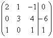 By the way, this is a fairly easy example, since the first column already has one zero, and there are fewer elementary transformations to perform.
The second feature is this. In all the examples considered, we placed either –1 or +1 on the “steps”. Could there be other numbers there? In some cases they can. Consider the system:  .
.
Here on the upper left “step” we have a two. But we notice the fact that all the numbers in the first column are divisible by 2 without a remainder - and the other is two and six. And the two at the top left will suit us! In the first step, you need to perform the following transformations: add the first line multiplied by –1 to the second line; to the third line add the first line multiplied by –3. This way we will get the required zeros in the first column.
Or another conventional example:  . Here the three on the second “step” also suits us, since 12 (the place where we need to get zero) is divisible by 3 without a remainder. It is necessary to carry out the following transformation: add the second line to the third line, multiplied by –4, as a result of which the zero we need will be obtained.
Gauss's method is universal, but there is one peculiarity. Confidently learn to solve systems using other methods (Cramer’s method, matrix method) you can literally the first time - there is a very strict algorithm. But in order to feel confident in the Gaussian method, you should “get your teeth into” and solve at least 5-10 ten systems. Therefore, at first there may be confusion and errors in calculations, and there is nothing unusual or tragic about this.
Rainy autumn weather outside the window.... Therefore, for everyone who wants more complex example for independent solution:
Example 5
Solve a system of 4 linear equations with four unknowns using the Gauss method. 
Such a task is not so rare in practice. I think even a teapot who has thoroughly studied this page will understand the algorithm for solving such a system intuitively. Fundamentally, everything is the same - there are just more actions.
Cases when the system has no solutions (inconsistent) or has infinitely many solutions are discussed in the lesson Incompatible systems and systems with a common solution. There you can fix the considered algorithm of the Gaussian method.
I wish you success!
Solutions and answers:
Example 2:
Solution
:
Let us write down the extended matrix of the system and, using elementary transformations, bring it to a stepwise form.
 Elementary transformations performed:
(1) The first line was added to the second line, multiplied by –2. The first line was added to the third line, multiplied by –1.
Attention!
Here you may be tempted to subtract the first from the third line; I highly recommend not subtracting it - the risk of error greatly increases. Just fold it!
(2) The sign of the second line was changed (multiplied by –1). The second and third lines have been swapped.
note
, that on the “steps” we are satisfied not only with one, but also with –1, which is even more convenient.
(3) The second line was added to the third line, multiplied by 5.
(4) The sign of the second line was changed (multiplied by –1). The third line was divided by 14.
Elementary transformations performed:
(1) The first line was added to the second line, multiplied by –2. The first line was added to the third line, multiplied by –1.
Attention!
Here you may be tempted to subtract the first from the third line; I highly recommend not subtracting it - the risk of error greatly increases. Just fold it!
(2) The sign of the second line was changed (multiplied by –1). The second and third lines have been swapped.
note
, that on the “steps” we are satisfied not only with one, but also with –1, which is even more convenient.
(3) The second line was added to the third line, multiplied by 5.
(4) The sign of the second line was changed (multiplied by –1). The third line was divided by 14.
Reverse:
Answer
:
![]() .
.
Example 4:
Solution
:
Let us write down the extended matrix of the system and, using elementary transformations, bring it to a stepwise form:

Conversions performed: (1) A second line was added to the first line. Thus, the desired unit is organized on the upper left “step”. (2) The first line multiplied by 7 was added to the second line. The first line multiplied by 6 was added to the third line.
With the second “step” everything gets worse , the “candidates” for it are the numbers 17 and 23, and we need either one or –1. Transformations (3) and (4) will be aimed at obtaining the desired unit (3) The second line was added to the third line, multiplied by –1. (4) The third line was added to the second line, multiplied by –3. The required item on the second step has been received. . (5) The second line was added to the third line, multiplied by 6. (6) The second line was multiplied by –1, the third line was divided by -83.
Reverse:
Answer :
Example 5:
Solution
:
Let us write down the matrix of the system and, using elementary transformations, bring it to a stepwise form:


Conversions performed: (1) The first and second lines have been swapped. (2) The first line was added to the second line, multiplied by –2. The first line was added to the third line, multiplied by –2. The first line was added to the fourth line, multiplied by –3. (3) The second line was added to the third line, multiplied by 4. The second line was added to the fourth line, multiplied by –1. (4) The sign of the second line was changed. The fourth line was divided by 3 and placed in place of the third line. (5) The third line was added to the fourth line, multiplied by –5.
Reverse:
![]()
Answer :